APPENDICES
APPENDIX 2-1.—DATA AND METHODS
The climate chapter of this assessment focuses on analyzing data from two main climate variables: temperature and precipitation. This scope was chosen based on the time, resources, and reliable data available for this assessment. Details about the data and methods of analysis used the climate chapter are below, organized by chapter section.
Montana’s Current Climate
To assess Montana’s current climate, we analyzed climate variable data provided as 3-decade averages by NOAA’s National Centers for Environmental Information (NOAAa undated). In the corresponding section of the chapter, we review average temperature and precipitation conditions from 1981-2010 as an indicator of current climate conditions.
Datasets used to determine climate normal:
-
Temperature.—The temperature analysis was derived from TopoWx (Topography Weather, commonly “twix”), a national temperature dataset of interpolated weather station observations developed at the University of Montana. TopoWx provides an 800-m, gridded minimum and maximum air temperature for 1948-2014, with measures of uncertainty (Oyler et al. 2015).
-
Precipitation.—For the precipitation normals, we performed our analysis with the widely used interpolation procedure from GRIDMET, from the University of Idaho (Abatzoglou 2013). GRIDMET derives the most accurate 4-km resolution interpolations of precipitation by combining 1) the desirable spatial attributes of gridded climate data from PRISM (Daly et al. 1994; Daly et al. 2017) with 2) reanalysis data from the North American Land Data Assimilation System (Xia et al. 2012a; Xia et al. 2012b). All precipitation measurements aggregate snow and rain to give the total water content in inches.
Historical Trend Analysis
We also looked at a broader set of historical trends, dating back to the start of the last century. We used standard statistical methods to analyze temperature and precipitation records spanning two periods: from 1950-2015 and 1900-2015.
Our analysis uses observational data from the US Climate Divisional Database (NOAAb undated). The data were treated to remove observational bias (e.g., station relocation, instrumentation changes, and observer practice changes) (Vose et al. 2014). Our approach included combining many stations to provide a more complete picture of historical changes for larger regions. In our analyses, we determined if a detectable trend exists for temperature and/or precipitation across either the seven climate divisions and/or the entire state.
As described in the Climate chapter, Montana includes seven NOAA climate divisions. For each climate division, we:
-
weighted the divisional values by their area to account for the unequal area of the climate divisions when determining statewide values (Karl and Koss 1984);
-
defined the seasons as a) winter—December, January, February, b) spring—March, April, May, c) summer—June, July, August, and d) fall—September, October, November;
-
computed monthly station temperature and precipitation values from the daily observations;
-
defined temperature minimums and maximums as the lowest and highest temperatures, respectively, recorded from each day averaged over the observed season;
-
defined precipitation to include the combination of rain and snow in inches of water content; and
-
evaluated trends in temperature or precipitation for significance using a least squares statistical regression, with change defined at the statistical probability level of p ≤ 0.05.
Our trend analysis used basic statistical methods to analyze records spanning two periods: from 1950-2015 and 1900-2015. The direction (increase or decrease) and significance of trends were generally similar for the two periods. Thus, the presentation of trends is confined to the period from 1950-2015.
Extreme Aspects of Montana's Climate
Along with analyzing historical trends in temperature and precipitation, we performed an analysis of changes in extreme climate events since the middle of last century. We performed our analysis of climate extremes using the CLIMDEX project (CLIMDEX undated), which provides a collection of global and regional climate data from multiple sources. CLIMDEX is developed and maintained by researchers at the Climate Change Research Centre and the University of New South Wales, in collaboration with the University of Melbourne, Climate Research Division of Environment Canada, and NOAA’s National Centers for Environmental Information. The CLIMDEX project aims to produce a global dataset of standardized indices representing the extreme aspects of climate.
Particular attention was placed on the changes in variables such as consecutive dry days, days of heavy precipitation, growing season length, frost days, number of cool days and nights, and the number of warm days and nights. Extreme precipitation events across the United States have increased in both intensity and frequency since 1901 (NCA 2014), including across both the High Plains and the northwestern US (many states combined), where studies have shown an increase in the number of days with extreme precipitation (NCA 2014). However, for our analysis at the state level we found no evidence of changes in extreme precipitation so it is not a variable of focus. In the Climate chapter, we report those variables that did change significantly (p<0.05) for Montana and, for perspective, the climate normals for these extremes for the periods 1951–1980 and from 1981-2010. We use the CLIMDEX definition of cool days as the percentage of days when maximum temperature is lower than 10% of the historical observations. We use the CLIMDEX definition of warm nights (and cool nights) as the number of days when minimum temperature is higher (lower) than a specified maximum (minimum) threshold defined by historical conditions.
Future Projections: Downscaling and Datasets
Scientists employ two methods for this downscaling of climate data from GCMs:
-
Dynamic downscaling.—Dynamic downscaling uses a limited-area, high-resolution model known as a regional climate model to derive finer-scale information. Boundary conditions from the GCMs drive the regional climate model. Dynamic downscaling is often the most accurate form of downscaling, but it is computationally intensive.
-
Statistical downscaling.—Statistical downscaling is less computationally intensive. It first derives relationships between historical, small-scale observations at high resolution and the larger-scale, GCMs climate variable. This statistical relationship can then be used in future projections to downscale the GCMs to higher resolutions to simulate local climate characteristics in the future.
For this climate assessment, we used a statistical downscaling method called the Multivariate Adaptive Constructive Analogs (MACA) (Abatzoglou and Brown 2012), and a training dataset called METDATA (Abatzoglou 2013). The dataset is freely available online from the University of Idaho (MACA undated). Other statistical downscaling methods and datasets are available, each with its own strengths and weaknesses, depending on such things as geography and topography of the study region.
Here we will refer to the full dataset we used as the MACAv2-METDATA dataset. The MACAv2-METDATA dataset includes the 20 CMIP5 models that make up our ensemble (Table A2-1). We employed only temperature and precipitation variables and they were downscaled to 4 km and daily resolution.
| Model Name | Model Country | Model Agency | Atmosphere Resolution (Lon x Lat) |
| bcc-csm1-1 | China | Beijing Climate Center, China Meteorological Administration | 2.8 deg x 2.8 deg |
| bcc-csm1-1-m | China | Beijing Climate Center, China Meteorological Administration | 1.12 deg x 1.12 deg |
| BNU-ESM | China | College of Global Change and Earth System Science, Beijing Normal University, China | 2.8 deg x 2.8 deg |
| CanESM2 | Canada | Canadian Centre for Climate Modeling and Analysis | 2.8 deg x 2.8 deg |
| CCSM4 | USA | National Center of Atmospheric Research, USA | 1.25 deg x 0.94 deg |
| CNRM-CM5 | France | National Centre of Meteorological Research, France | 1.4 deg x 1.4 deg |
| CSIRO-Mk3-6-0 | Australia | Commonwealth Scientific and Industrial Research Organization/Queensland Climate Change Centre of Excellence, Australia | 1.8 deg x 1.8 deg |
| GFDL-ESM2M | USA | NOAA Geophysical Fluid Dynamics Laboratory, USA | 2.5 deg x 2.0 deg |
| GFDL-ESM2G | USA | NOAA Geophysical Fluid Dynamics Laboratory, USA | 2.5 deg x 2.0 deg |
| HadGEM2-ES | United Kingdom | Met Office Hadley Center, UK | 1.88 deg x 1.25 deg |
| HadGEM2-CC | United Kingdom | Met Office Hadley Center, UK | 1.88 deg x 1.25 deg |
| inmcm4 | Russia | Institute for Numerical Mathematics, Russia | 2.0 deg x 1.5 deg |
| IPSL-CM5A-LR | France | Institut Pierre Simon Laplace, France | 3.75 deg x 1.8 deg |
| IPSL-CM5A-MR | France | Institut Pierre Simon Laplace, France | 2.5 deg x 1.25 deg |
| IPSL-CM5B-LR | France | Institut Pierre Simon Laplace, France | 2.75 deg x 1.8 deg |
| MIROC5 | Japan | Atmosphere and Ocean Research Institute (The University of Tokyo), National Institute for Environmental Studies, and Japan Agency for Marine-Earth Science and Technology | 1.4 deg x 1.4 deg |
| MIROC-ESM | Japan | Japan Agency for Marine-Earth Science and Technology, Atmosphere and Ocean Research Institute (The University of Tokyo), and National Institute for Environmental Studies | 2.8 deg x 2.8 deg |
| MIROC-ESM-CHEM | Japan | Japan Agency for Marine-Earth Science and Technology, Atmosphere and Ocean Research Institute (The University of Tokyo), and National Institute for Environmental Studies | 2.8 deg x 2.8 deg |
| MRI-CGCM3 | Japan | Meteorological Research Institute, Japan | 1.1 deg x 1.1 deg |
| NorESM1-M | Norway | Norwegian Climate Center, Norway | 2.5 deg x 1.9 deg |
Literature Cited
Abatzoglou JT. 2013. Development of gridded surface meteorological data for ecological applications and modelling. International Journal of Climatology 33:121–31.
Abatzoglou JT, Brown TJ. 2012. A comparison of statistical downscaling methods suited for wildfire applications. International Journal of Climatology 32:772–80.
CLIMDEX. [undated]. CLIMDEX—datasets for indices of climate extremes [website]. Available online http://climdex.org/. Accessed 2017 Mar 6.
Daly C, Neilson RP, Phillips DL. 1994. A statistical-topographic model for mapping climatological precipitation over mountainous terrain. Journal of Applied Meteorology and Climatology 33:140-58.
Daly C, Slater M, Roberti JA, Laseter S, Swift L. 2017. High-resolution precipitation mapping in a mountainous watershed: ground truth for evaluating uncertainty in a national precipitation dataset. International Journal of Climatology 37:124-37. doi:10.1002/joc.4986.
Karl T, Koss WJ. 1984. Regional and national monthly, seasonal, and annual temperature weighted by area, 1895-983. Historical Climatology Series 4-3. Asheville NC: National Climatic Data Center. 38 p.
[MACA] Multivariate adaptive constructed analogs. [undated]. MACA statistically downscaled climate data from CMIP5 [website]. Available online http://maca.northwestknowledge.net/. Accessed 2016 Oct 16.
[NCA] National Climate Assessment. 2014. In: Melillo JM, Richmond T, Yohe GW, editors. Climate change impacts in the United States: the third national climate assessment. Washington DC: US Global Change Research Program. 841 p. doi:10.7930/J0Z31WJ2.
[NOAAa] National Oceanic and Atmospheric Administration. [undated]. Climate normals [website]. Available online https://www.ncdc.noaa.gov/data-access/land-based-station-data/land-based.... Accessed 2017 Mar 6.
[NOAAb] National Ocenaic and Atmorspheric Administration. [undated]. Climate at a glance [website]. Available online: www.ncdc.noaa.gov/cag/. Accessed 2017 Mar 6.
Oyler JW, Ballantyne A, Jencso K, Sweet M, Running SW. 2015. Creating a topoclimatic daily air temperature dataset for the conterminous United States using homogenized station data and remotely sensed land skin temperature. International Journal of Climatology 35:2258–79.
Vose RS, Applequist S, Durre I, Menne MJ, Williams CN, Fenimore C, Gleason K, Arndt D. 2014. Improved historical temperature and precipitation time series for US climate divisions. Journal of Applied Meteorology and Climatology 53(5):1232-51. Available online http://dx.doi.org/10.1175/JAMC-D-13-0248.1. Accessed 2017 May 10.
Xia Y, Mitchell K, Ek M, Sheffield J, Cosgrove B, Wood E, Luo L, Alonge C, Wei H, Meng J, Livneh B, Lettenmaier D, Koren V, Duan Q, Mo K, Fan Y, Mocko D. 2012a. Continental-scale water and energy flux analysis and validation for the North American Land Data Assimilation System project phase 2 (NLDAS-2): 1. Intercomparison and application of model products. Journal of Geophysical Research 117:D03109. doi:10.1029/2011JD016048.
Xia, Y, Mitchell K, Ek M, Sheffield J, Cosgrove B, Wood E, Luo L, Alonge C, Wei H, Meng J, Livneh B, Lettenmaier D, Koren V, Duan Q, Mo K, Fan Y, Mocko D. 2012b. Continental-scale water and energy flux analysis and validation for North American Land Data Assimilation System project phase 2 (NLDAS-2): 2. Validation of model-simulated streamflow. Journal of Geophysical Research 117:D03110. doi:10.1029/2011JD016051.
APPENDIX 2-2.—OTHER IMPORTANT TELECONNECTIONS
As mentioned in the body of the report, understanding teleconnections is important for understanding medium-term (weeks to decades) variations in Montana’s weather and climate. The report details the two most important teleconnections to Montana’s climate (El Niño-Southern Oscillation and Pacific Decadal Oscillation). Here we provide an overview of three other teleconnections that play a part in Montana’s climate and weather:
-
The Pacific-North American Teleconnection Pattern.—The Pacific-North American teleconnection is a short-term (<1 month) pattern of variation in the polar jet stream. It affects storms moving from the Pacific Ocean into the northwestern US. The Pacific-North American teleconnection is strongest in the winter, when it influences temperature and, to a lesser extent, precipitation in Montana. During positive phases, a persistent high-pressure system blocking ridges develops over the northern Rocky Mountains, steering Pacific storms northward and leading to decreased precipitation and generally higher temperatures in Montana. During the negative phase the pattern is reversed, and a weakened high-pressure system over the Northern Rockies allows the intrusion of maritime polar and Arctic air masses, leading to cooler temperatures and increased precipitation (Leathers et al. 1991; Leathers and Palecki 1992).
-
Madden-Julian Oscillation.—The Madden-Julian Oscillation connects the uplift of moisture-laden air masses in the Pacific Ocean with global atmospheric circulation, leading to precipitation for periods of 30-60 days (Zhang 2013). Although its strongest effects center around the equator, the Madden-Julian Oscillation also has a significant impact on the West Coast of North America, where it has been associated with unusually heavy rainfall and major flooding events (Bond and Vecchi 2003; Zhou et al. 2012). These effects often continue into the mountains of western Montana, where they can contributed heavy precipitation (Becker et al. 2011; Zhou et al. 2012).
-
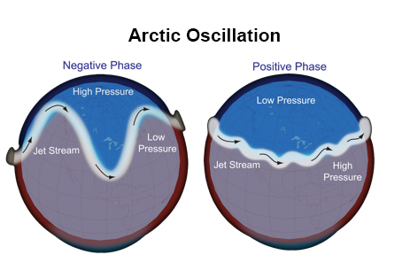
Arctic Oscillation.—The Arctic Oscillation refers to opposing fluctuations in atmospheric pressure over the north polar region and mid latitudes (a similar pattern occurs in the Southern Hemisphere). These fluctuations occur over weeks to months. They influence the flow of the mid-latitude jet stream, and thus its ability to move polar air into the mid latitudes. The Arctic Oscillation has a strong influence on North American winter temperatures and, to a lesser extent, precipitation. During the positive phase of the Arctic Oscillation, the jet stream shows less sinuosity (Figure A2-2). As a result, little Arctic air moves south, which in turn leads to drier and often warmer conditions in the western US, plus a small increase in precipitation in the Pacific Northwest. During the negative phase, the jet stream shows more sinuosity, polar air penetrates to lower latitudes, and Pacific storms are forced to the south. These changes lead to cooler temperatures and increased precipitation in Montana (Thompson and Wallace 2001).
|
|
| Figure A2-2: The Arctic Oscillation has a strong influence on North American winter temperatures and, to a lesser extent, precipitation. During the positive phase, the jet stream shows less sinuosity and Arctic air is prevented from moving south, leading to drier and often warmer conditions in the western US and a small increase in precipitation in the Pacific Northwest. During the negative phase, the jet stream shows more sinuosity, polar air penetrates into the lower latitudes, and pacific storms are forced to the south. This leads to both cooler temperatures and increased precipitation in Montana. |
Literature Cited
Becker EJ, Berbery EH, Higgins RW. 2011. Modulation of cold-season US daily precipitation by the Madden-Julian Oscillation. Journal of Climate 24(19):5157-66.
Bond NA, Vecchi GA. 2003. The Influence of the Madden—Julian Oscillation on precipitation in Oregon and Washington. Weather Forecast 18:600–13.
Leathers DJ, Brent Y, Palecki MA. 1991. The Pacific/North American teleconnection pattern and United States climate. Part I: Regional temperature and precipitation associations. Journal of Climate 4:517–28.
Leathers DJ, Palecki MA. 1992. The Pacific/North American teleconnection pattern and United States climate. Part II: Temporal characteristics and index specification. Journal of Climate 5:707–16.
Thompson DWJ, Wallace JM. 2001. Regional climate impacts of the Northern Hemisphere annular mode. Science 293:85–9.
Zhang C. 2013. Madden-Julian Oscillation: bridging weather and climate. Bulletin of the American Meteorological Society 94:1849–70.
Zhou S, L’Heureux M, Weaver S, Kumar A. 2012. A composite study of the MJO influence on the surface air temperature and precipitation over the continental United States. Climate Dynamics 38:1459–71.
APPENDIX 3.1—FOCAL RIVER INFORMATION
To best represent the influence of climate variations on water resources, the Water chapter of the 2017 MCA focuses on eight rivers and their watersheds (note that some watersheds—for example, Poplar River and others—extend beyond the state boundaries). These focal rivers and watersheds, chosen across the state’s seven National Oceanic and Atmospheric (NOAA) climate divisions, include:
- Climate division 1 – Clark Fork River at Saint Regis
– Middle Fork of the Flathead River at West Glacier
- Climate division 2 – Missouri River at Toston
- Climate division 3 – Marias River near Shelby
- Climate division 4 – Musselshell River at Mosby
- Climate division 5 – Yellowstone River at Billings
- Climate division 6 – Poplar River near Poplar
- Climate division 7 – Powder River near Locate
More information on these focal rivers is provided in Table A3-1 and the corresponding text below.
| Climate Division | Focal River | Area (square miles) | Period of Flow Record | Years of Flow Record |
| 1* | Clark Fork at St. Regis | 10,728 | 1930-2016 | 86 |
| 1* | Middle Fork of the Flathead at West Glacier | 1,125 | 1941-2015 | 74 |
| 2* | Missouri at Toston | 14,641 | 1942-2015 | 73 |
| 3 | Marias near Shelby | 2,716 | 1912-2015 | 103 |
| 4 | Musselshell at Mosby | 7,784 | 1931-2015 | 84 |
| 5 | Yellowstone at Billings | 11,414 | 1929-2015 | 86 |
| 6 | Poplar near Poplar | 3,140 | 1909-2015** | 72 |
| 7 | Powder near Locate | 13,060 | 1939-2015 | 76 |
* There is a small part of Climate Division 1 that is located on the east side of the Continental Divide and a small part of Climate Division 2 located on the west side of the Continental Divide (see Water chapter Figure 3-5).
** Missing years over that period, annual data available: 1909-1924, 1948-1969, 1976-1979, 1982-2015.
Clark Fork River at St. Regis
[86 years of record; drainage area = 10,728 square miles]
Summary: This gage is located upstream from the confluence of the Clark Fork and Flathead Rivers. It measures streamflow from largely unregulated tributaries (Upper Clark Fork, Bitterroot, Blackfoot). Land uses are predominantly agricultural with a majority of the valley bottoms used for cattle ranching. There are large areas of irrigated acreage in the Bitterroot, Upper Clark Fork and Flint Creek drainages. This gage site is located upstream of the major hydroelectric dams on the Clark Fork. There is also significant urban development in the Missoula Valley.
Reservoirs: No large reservoirs exist above this gage site, although numerous small reservoirs are present in headwater tributaries.
- Painted Rocks Reservoir (West Fork of the Bitterroot)
- Georgetown Lake (Flint Creek)
- East Fork Reservoir (East Fork of Rock Creek)
Middle Fork of the Flathead River at West Glacier
[77 years of record; drainage area = 1,125 square miles]
Summary: The Middle Fork of the Flathead gage at West Glacier is located near the confluence of the Middle Fork and the South Fork (which form the Flathead proper). The majority of the land area in the Middle Fork Basin is protected as part of Glacier National Park or the Bob Marshall Wilderness. There is very limited human development of water resources in this Basin. Of all the sites in this assessment, this one could be considered to be the most hydrologically “pristine.”
Reservoirs: There are no small or large reservoirs located in the Basin.
Missouri River at Toston
[82 years of record; drainage area = 14,641 square miles]
Summary: The Missouri River gage at Toston encompasses a substantial drainage area and is located downstream of the confluence of all three of the major headwaters of the Missouri (Madison, Jefferson, and Gallatin Rivers). Land uses upstream of the Toston gage are predominantly agricultural, with significant urban development in the Gallatin Valley proximate to Bozeman. Irrigated agriculture is concentrated in the Jefferson and Gallatin Basins and significantly impacts flows at the confluence of the Missouri. The Jefferson and lower Gallatin rivers are heavily utilized for irrigation and are frequently dewatered during the summer growing season.
Reservoirs: Relative to the size of the drainage area at the Toston gage, there are limited large-scale water storage facilities upstream from the gage site and the influence of upstream dams on flow are relatively minor. The large reservoirs on the Madison River are primarily utilized for hydropower with smaller scale reservoirs (used for irrigation) present in the Ruby and Beaverhead drainages (part of the Jefferson River Basin).
- Hebgen Dam (Madison River)
- Ennis Lake (Madison River)
- Ruby Reservoir (Ruby River)
- Clark Canyon Dam (Beaverhead River)
Marias River near Shelby
[111 years of record; drainage area= 2,716 square miles]
Summary: The Marias River (a tributary of the Missouri) is formed by the confluence of Cut Bank Creek and the Two Medicine River in Glacier County. This gage is located upstream of the largest reservoir in the basin, Tiber Dam (Lake Elwell). Land uses upstream of the gage are predominantly farming (both irrigated and dryland) and ranching. A large irrigation project on the Blackfeet Reservation upstream of Shelby modifies flows at the gage site.
Reservoirs: The Bureau of Indian Affairs manages several reservoirs on the Blackfeet Reservation for flood control and irrigation storage. These reservoirs are located in both Cut Bank Creek and Two Medicine River drainages and the headwaters of the Marias River system. The federal government initiated the “Blackfeet Irrigation Project” in 1907 with the goal of irrigating approximately 100,000 acres on the Reservation through a series of reservoirs and canals.
- Mission Dam (Spring Creek)
- Lower Two Medicine Dam (Two Medicine River)
- Swift Dam (Birch Creek)
- Four Horns Dam (Badger Creek)
Musselshell River at Mosby
[84 years of record; drainage area= 7,784 square miles]
Summary: The Musselshell River gage at Mosby is located at the lower end of the watershed, approximately 60 river miles from the confluence at Fort Peck Lake. Although the Musselshell flows a significant distance (approximately 350 miles), the volume of its flows is relatively small. All the major tributaries to the Musselshell are absorbed upstream of Mosby. The Musselshell is formed approximately 300 miles upstream of Mosby at the confluence of the North and South Forks of the Musselshell. Land uses upstream of the gage are predominantly agricultural and the river experiences frequent dewatering during the summer due to irrigation demands (especially from Martindale to Mosby). Irrigation significantly impacts flows on the Musselshell.
Reservoirs: There are numerous large and small-scale reservoirs upstream of the Mosby gage site that impact flows on the Musselshell. All the reservoirs were constructed to provide water for irrigation.
- Petrolia Reservoir (Flatwillow Creek)
- Deadman’s Basin Reservoir (Musselshell River)
- Bair Reservoir (N. Fork Musselshell River)
- Martinsdale Reservoir (Musselshell River)
Yellowstone River at Billings
[88 years of record; drainage area= 11,414 square miles]
Summary: The Yellowstone River gage at Billings is located downstream of the confluence of the Boulder, Stillwater, Shields, Rosebud and Clarks Fork Rivers. The gage is located upstream of the Yellowstone’s largest tributary, the Bighorn River, as well as the Tongue and Powder Rivers. A part of the Yellowstone’s headwaters are located in Wyoming in Yellowstone National Park. Land uses upstream of this gage are predominantly agricultural with significant urban development in the Yellowstone Valley between Laurel and Lockwood. Due in large part to the geography of the Yellowstone River Valley (relatively narrow floodplain), the river is not over-appropriated like many of the other systems in Montana. Large parts of the land area in the upper Yellowstone Basin are classified as National Park, federal Wilderness Areas, or Forest Service lands. The Yellowstone’s headwaters on the Beartooth Plateau also contain the highest elevations in Montana.
Reservoirs: The main stem of the Yellowstone River is considered the longest free-flowing river in the contiguous US (692 miles from the headwaters to the confluence with the Missouri). There are however, small reservoirs in some of the headwaters tributaries. The reservoirs in the headwaters are used for both hydropower and irrigation. The large reservoirs in the Basin are located downstream of the Yellowstone gage, on the Bighorn and Tongue Rivers.
- Glacier Lake Dam (Rock Creek)
- Mystic Lake (West Rosebud Creek)
- Cooney Reservoir (Red Lodge Creek)
Poplar near Poplar
[78 years of record; drainage area= 3,140 square miles]
Summary: The Poplar River gage near Poplar is located within 2 miles of the confluence of the Poplar and Missouri Rivers, and is below all of the major tributaries to the Missouri. Although the Poplar flows a significant distance of 167 miles, the river flows through an arid landscape and discharge at the mouth is relatively low (i.e., approximately 100 cubic feet per second). The period of gaged record at this location contains gaps; coverage includes the years 1909-1924, 1948-1969, 1976-1979, and 1982-present. It is important to note that both of the major tributaries of the Poplar River (the East Fork and West Fork) originate in southern Saskatchewan in Canada. Land uses upstream of the gage site are primarily agricultural; mostly dryland, but with some irrigated (approximately 8000 irrigated acres). There is also a large coal mine located upstream near the headwaters of the Poplar River in Canada.
Reservoirs: There are no large reservoirs in the Poplar Basin although there are numerous small scale stock watering ponds.
Powder River near Locate
[78 years of record; drainage area= 13,060 square miles]
Summary: The Powder River near Locate is located approximately 30 miles upstream from the confluence of the Powder and Yellowstone Rivers. The Powder River headwaters are located in the Bighorn Mountains of Wyoming and most of the basin’s water is sourced in Wyoming. The river and its drainage basin are relatively large (the river flows for 375 miles). Land uses upstream of the gage site are primarily ranchlands with some irrigated farmland confined to the Powder River Valley bottom. The Powder River Basin is also the largest coal producing region in the US, supplying 40% of the country’s coal. Water use on the river is governed under the 1950 Yellowstone River Compact between Montana, Wyoming, and North Dakota. According to the treaty, Montana receives 58% (Wyoming 42%) of flows measured at the last point of diversion directly above the Yellowstone confluence (near Terry, MT).
Reservoirs: The Powder River Basin contains a several large reservoirs in the Wyoming part of the watershed in the Bighorn Mountains. Lake DeSmet is the largest storage facility in the Basin although it does not significantly impact streamflow volumes.
- Lake DeSmet (Shell Creek)
- Kearney Lake Reservoir (Piney Creek)
- Willow Park Reservoir (South Piney Creek)
- Cloud Peak Reservoir (South Piney Creek)
APPENDIX 3-2.—SNOWPACK ANALYSIS
To analyze trends in Montana snowpack we utilized the USDA Natural Resources Conservation Service (NRCS) Snow Course database for Montana. This database contains Snow Course records over the period 1935-2016. There are approximately 100 Snow Course stations with data available in Montana. Below we provide more detail about our analysis of the NRCS Snow Course data.
| Relative Location | Period of snow course record | Elevation (feet) | Max # of snow course stations |
| West of the Continental Divide | 1937-2016 | >6000 | 22 |
| <6000 | 29 | ||
| East of the Continental Divide | 1936-2016 | >7000 | 25 |
| <7000 | 24 |
Organizational Structure
- Stations with less than 20 years of continuous April 1 SWE (snow water equivalent) measurements were not used.
- Snow Course data was grouped by (a) location relative to the Continental Divide and (b) elevation.
- (a) Continental Divide - East or West
- (b) Elevation - above or below 7,000 feet (East) or 6,000 feet (West)
- Elevations were chosen to distribute stations somewhat equally across elevation groups.
Normalization
- To normalize Snow Course data, z-scores were computed for each snow course record.
- z-score = (long term April 1 SWE average – annual April 1 SWE) / (long term April 1 SWE standard deviation)
- This produced a record of unitless snowpack (normalized records have a mean of 0 and standard deviation of 1)
- After normalizing individual station records, the data were nested by elevation and relative location to the Continental Divide (nested values averaged).
Converting Normalized Data to Values with Units
- Data were rescaled to produce values in units of SWE (inches).
- To convert the normalized SWE data for each year of the record:
- Average snow depth (SD) and April 1 SWE values were calculated for all Snow Course stations over the period of record. This was calculated from the raw April 1 SWE data.
- Regional mean SD and April 1 SWE (using the data from the previous step) values were then computed for all groups of stations (i.e., E/W of the Continental Divide, above or below 6,000 or 7,000 feet).
- To adjust the z-score to equal the observational record:
- The z-score value for each site at every year was multiplied by the regional mean SD and that value was added to the regional mean average April 1 SWE.
- It is important to note that there were multiple regional mean SDs and averages (computed for each grouping E/W of the Continental Divide or above and below 6,000 or 7,000 feet).
- The rescaled regional data was then averaged by year to compile the regional graphs used in the MCA.
Data QA/QC Issues
- April 1 SWE measurements are typically taken close to the April 1st date but are not always on April 1st (can be taken a week or so before or after).
- There are potential issues with site consistency at Snow Course locations due to forest succession, wildfire, etc.
- The number of snow survey sites used for a given annual estimate varied across years.
- Potential biases exist due to the distribution of Snow Course station elevations.
APPENDIX 5-1.—MONTANA CROP AND LIVESTOCK STATISTICS BY REGION
Table A5-1: Montana crop and livestock statistics by region. (NASS 2015)
| PLANTED | HARVESTED | YIELD | PRODUCTION | |
| Acres | Acres | Bushels, Tons, or Cwt | Bushels, Tons, or Cwt | |
| NORTHWESTERN | ||||
| Winter Wheat | 12,000 | 10,600 | 65.4 | 693,000 |
| Spring Wheat | 24,700 | 24,100 | 68.5 | 1,650,000 |
| Barley | --- | --- | --- | --- |
| Oats | 2,500 | 1,100 | 107.3 | 118,000 |
| Corn (Grain and Silage) | --- | 1,500 | ---/23.5 | ---/35,000 |
| Potatoes | 2,400 | 2,320 | 291.0 | 674,000 |
| Sugar Beets | --- | --- | --- | --- |
| NORTH CENTRAL | ||||
| Winter Wheat | 1,435,000 | 1,300,000 | 41.8 | 54,308,000 |
| Spring Wheat | 1,078,200 | 1,055,400 | 36.1 | 38,115,000 |
| Barley | 519,000 | 476,000 | 55.4 | 26,360,000 |
| Oats | 7,300 | 1,900 | 61.6 | 117,000 |
| Corn (Grain and Silage) | 11,000 | 10,800 | 86.3/20.0 | 751,000/42,000 |
| Potatoes | --- | --- | --- | --- |
| Sugar Beets | --- | --- | --- | --- |
| NORTHEASTERN | ||||
| Winter Wheat | 307,800 | 233,700 | 34.1 | 7,976,000 |
| Spring Wheat | 1,587,800 | 1,560,200 | 32.5 | 50,765,000 |
| Barley | 71,700 | 37,700 | 52.6 | 1,983,000 |
| Oats | 17,200 | 4,700 | 54.5 | 256,000 |
| Corn (Grain/Silage) | 36,000 | 35,400 | 89.3/19.5 | 2,160,000/219,000 |
| Potatoes | --- | --- | --- | --- |
| Sugar Beets | 16,300 | 16,000 | 30.7 | 491,000 |
| CENTRAL | ||||
| Winter Wheat | 415,000 | 397,100 | 39.8 | 15,790,000 |
| Spring Wheat | 156,000 | 151,900 | 37.4 | 5,677,000 |
| Barley | 168,000 | 142,000 | 53.9 | 7,650,000 |
| Oats | 6,600 | 2,800 | 73.6 | 206,000 |
| Corn (Grain/Silage) | 10,000 | 9,900 | 46.0/21.0 | 290,000/75,000 |
| Potatoes | 1,500 | 1,490 | 391.0 | 583,000 |
| Sugar Beets | --- | --- | --- | --- |
| SOUTHWESTERN | ||||
| Winter Wheat | 26,500 | 24,100 | 41.1 | 990,000 |
| Spring Wheat | 37,300 | 36,100 | 66.6 | 2,406,000 |
| Barley | 53,400 | 40,000 | 72.5 | 2,900,000 |
Basis is the difference between futures market price and local price. A futures contract is a legally binding agreement to sell or buy a specific commodity for a specified price at a specified time in the future. Futures contracts are established and exchanged at a single central market (e.g., the Chicago Mercantile Exchange). Because futures contracts for major commodities—including wheat—are established by many individuals and agribusinesses from across the US and around the world, the price of a futures contract reflects a highly-informed estimate of future commodity prices.
Futures contracts are also used extensively by grain handling facilities to hedge their price risks when establishing local (forward) contracts with farmers for grain delivery. As such, prices that agricultural producers observe are highly—but not perfectly—correlated to those in the futures market. Basis represents that imperfect relationship between the local and futures contract prices. These differences occur for a number of reasons, including specificities in a crop's local supply and demand conditions, crop quality, and other characteristics that differentiate the crop from the standards set by a futures contract, transportation costs, and other factors.
Basis can be used to assess differential impacts of climate change on local and global agricultural commodity markets because it helps characterize the manner, in which Montana-specific crop prices (reflective of local production conditions) are related to prices in futures markets (reflective of global conditions). For example, if climate change leads to basis becoming more negative (or less positive) relative to historical averages—that is, the local price decreases relative to the futures price—this would imply that the impacts of the climate changes likely affected local prices more adversely than global prices. Conversely, rising basis would indicate that local production and marketing conditions were less impacted (adversely) by climate change relative to global conditions. Therefore, basis enables the analysis of wheat economics at a local level while accounting for global market conditions.
We describe two principal ways in which climate change can impact the economics of Montana's crop industry:
Increased Production and Marketing Uncertainty
Agricultural production's dependency on weather conditions makes the sector unavoidably exposed to uncertainty in both commodity crop yields and prices. Yield uncertainty (also commonly referred to as crop production risk) is the result of unpredictable weather patterns that manifest as drought, floods, hail, and other extreme weather events that significantly reduce crop yields. While these dangers are not new to the agricultural sector, climate change can exacerbate the uncertainty of both when these events occur and the magnitude of their adverse impacts. Price uncertainty refers to the fact that producers are unable to perfectly predict the price they will receive for their crop at the time that these producers are seeding. These temporal risks are a result of the combination of regional and global production uncertainties and the varying demand for certain agricultural products.
US crop producers are able to partially reduce production risks by purchasing annual crop insurance products. While crop insurance does not directly reduce production uncertainties, it does offer producers some level of compensation for economic losses resulting from unexpected yield losses. Regardless, crop insurance is often perceived by producers as the main mechanism to mitigate climate change impacts. For example, in 2016, over 95% of planted wheat acres in Montana were insured by a federally subsidized crop insurance product (USDA-RMA 2016). Managing price risk can take on several forms. The most used price risk management tool is a contract that "locks in" a price that a farmer is guaranteed to receive at delivery of a crop. A futures contract and forward contract are two of the most common ways that a farmer can establish a guaranteed price at the time of delivery. Futures contracts are established on a centralized futures contract exchange (e.g., Chicago Mercantile Exchange and Minneapolis Grain Exchange) between a producer and an unknown buyer. Forward contracts are agreed upon between a producer and a known local grain elevator.
Regardless of the price management tool chosen by a farmer, both the futures and forward contracts are still subject to basis risk, which is the result of production and marketing differences between local and global production regions. Basis risk results from unexpected deviations from long-run basis trends. Although basis risks are much smaller than price risk, neither agricultural producers nor procurers have many fewer opportunities to hedge against basis risk. A farmer using the futures market to mitigate the risk of grain price fluctuations will be directly subject to basis risk (and the costs associated with that risk). Alternatively, when a farmer establishes a forward contract with a local grain elevator, the farmer transfers both price risk and local basis risk to the grain elevator. However, because both risks (and associated costs) are transferred to the grain elevator, the grain elevator enacts a surcharge on a forward contract as a means of risk mitigation for the grain elevator3. This surcharge is typically in the form of offering a producer a lower price than if the producer established a futures contract and directly took basis risk.
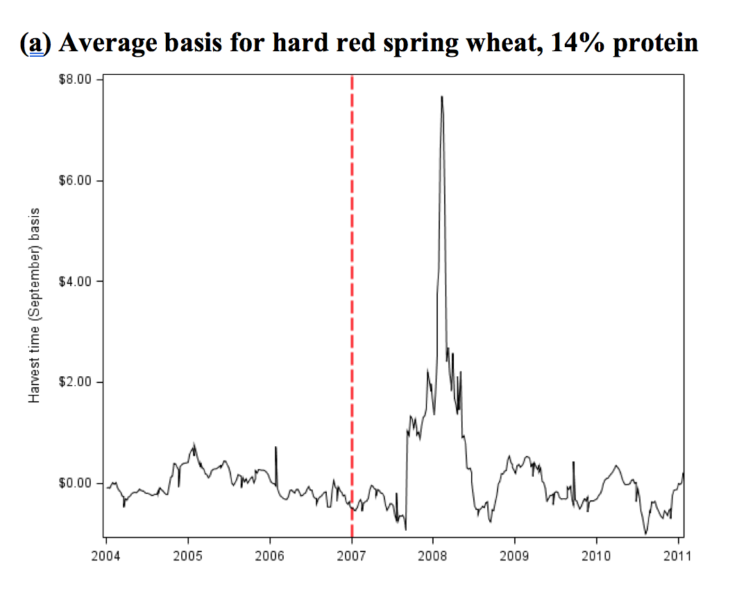
Basis risk for hard red spring wheat and hard red winter wheat in the northern US has been relatively small but increased since the mid 2000s (Figure A5-2.1). Furthermore, basis has become more volatile. Throughout 2004-2007 basis generally followed a seasonal pattern, but the pattern changed in the fall of 2007. This is partially explained by substantial change in small grain crop production in the Northern Plains due to changes in crop profitability and an introduction of short-season corn varieties that have enabled traditional wheat-producing regions to replace part of wheat production with these new corn varieties (Bekkerman et al. 2016). These short-season corn varieties have been able to take hold due to climate change creating a longer growing season and shorter winter. This has resulted in a decrease in the production and stock of small grains, which in turn has likely increased price uncertainty in these small local markets (and basis) (Bekkerman et al. 2016).
 |
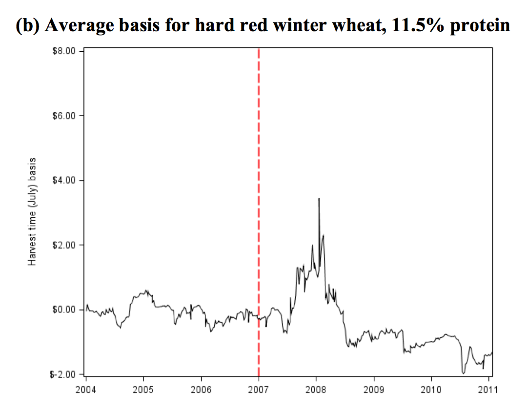 |
| Figure A5-2.1: Average basis for hard red spring wheat, 14% protein (a) and average basis for hard red winter wheat, 11.5% protein (b). Figure from Bekkerman et al. 2016. |
Regardless of the reasons for the increase in basis volatility, increased basis uncertainty decreases farmers’ ability to manage price uncertainty using traditional tools. In futures markets, increased basis uncertainty directly increases farmers’ cost of price risks. Taylor M. et al. (2014) show that increased basis volatility also increase costs for farmers who use forward contracts. Their study evaluated the structural change in forward contracting costs for Kansas wheat, in which they found that an increase in basis volatility along with the information available in the market as harvest approaches, are among several factors that increase forward contracting costs for farmers. When elevators are less certain about future harvest prices (and, thus, basis), they pass on the increased risk of losing money on a forward contract (due to an inaccurate basis prediction) by increasing the amount of risk premium that they charge the farmer. That is, the more uncertain an elevator is about future prices, the higher the risk surcharge that they pass on to farmers, and therefore, the lower the price that a farmer will receive for their grain. The comparison of observed and predicted forward contracting costs over time (Figure A5-2.2) make it clear that the increases in the risk premiums charged to farmers who establish forward contracts corresponds closely to increases in basis volatility since 2007.
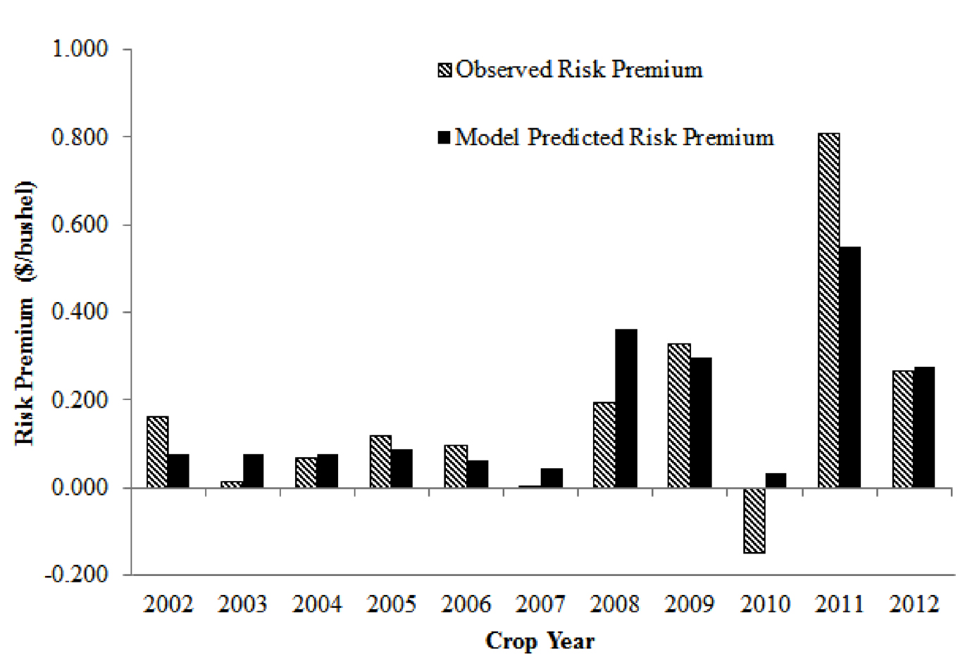 |
| Figure A5-2.2: The relative comparison of observed and predicted forward contracting costs over time. Figure from Taylor et al. 2014. |
It is worth noting that forward contracts are typically priced higher than normal in the year following a negative cost year—a negative cost year meaning the farmers received more for their forward contract grain than if they had waited to sell their grain at harvest (Figure A5-2.2). This implies that past actual returns to the grain elevator could potentially be more important in determining decisions than expectations of future returns, and is supported by a finding in a study of cattle feeder behavior conducted by Kastens and Schroeder (1995).
Continued climate change can further exacerbate increased basis volatility. Moreover, it can do so through its impacts on both local production and marketing conditions (i.e., the local price), through impacts on global conditions (i.e., the futures contract price), or through both local and global channels. Farmers who do not actively manage price risk will be subject to even greater uncertainty about market prices, and can suffer more dramatic losses during low price years. Even farmers who do use futures or forward contracts to hedge price uncertainty are likely to obtain lower prices because increased basis risks will be transferred to increases in risk costs.
Impacts on Wheat Quality and Product Differentiation
Several other marketing factors—unique to the northern US wheat-producing region—could be impacted by climate change and affect economic returns from wheat production. Wheat produced in Montana and other northern US states is differentiated by class (hard red spring and hard red winter) and level of protein, which are both important marketable characteristics for producing different wheat-based consumer products. Therefore, wheat prices depend on both local supply and demand, transportation factors, and storage availability conditions as well as the scarcity of a particular characteristic (such as sufficient protein levels) across other wheat production regions (e.g., the central and southern Great Plains). If winter wheat grown in the southern US has a lower protein content, protein premiums for northern spring and winter wheat are likely to be higher, implying that Montana producers who can supply the higher-protein wheat would receive a higher price for their wheat. However, these premiums can disappear if favorable production conditions in the southern US region lead to saturation of a high-protein wheat market (Kastens and Schroeder 1994).
The relationship between wheat quality levels and prices play an important part in the economics of wheat in Montana and can influence a farmer’s choice for what kind of wheat to grow as well as other production strategies. For example, winter wheat generally has a higher yield than spring wheat, but spring wheat has a higher protein content than winter wheat and therefore can receiver a higher protein premium to offset the smaller yield.
Climate change can impact Montana producers’ abilities to take advantage of price premiums that result from market demand for high quality wheat. As climate change continues to affect general production conditions—bringing warmer and wetter (precipitation in the form of rain, not snow) winters, and hotter and drier summers—higher-protein hard red spring wheat may not continue to be an economically viable crop to be produced by northern US farmers. As such, there is an expected shift away from spring wheat and toward winter wheat production (Power and Power 2016). If this is the case, then Montana farmers may lose an important competitive advantage in producing and marketing a higher priced quality-differentiated product.
The exact effect climate change will have on wheat yield is still unpredictable. A study on the overall impact of climate change on crops grown in the Flathead Valley of Montana highlights the difficulties in quantifying climate change’s impact on Montana agriculture (Prato and Qui 2013). The study found that the net crop return per hectare would decrease by 24% and the net farm income overall would decrease by 57%. The range of the predicted impacts of climate change, however, is much greater, as soil type, climate scenarios, and mitigation methods all impact the outcome of projected climate change on crop yield. Depending on the soil type, increase in CO2 fertilization and crop type, it is possible that some crops, such as winter wheat, might see an increase in yield from climate change. The only certain change is greater uncertainty for crop yield and price.
Literature Cited
Bekkerman A, Brester GW, Taylor M. 2016. Forecasting a moving target: the roles of quality and timing for determining northern US wheat basis. Journal of Agricultural and Resource Economics 41(1):25-41.
Kastens T, Schroeder TC. 1994. Cattle feeder behavior and feeder cattle placements. Journal of Agricultural and Resource Economics 19(2):337-348.
Power TM, Power DS. 2016. The impact of climate change on Montana’s agricultural economy. Prepared for Montana Farmers’ Union by Power Consulting Inc. 28 p. Available online http://montanafarmersunion.com/wp-content/uploads/2016/02/FINAL_Impact_Climate_Change_MT_Ag_Econ_Power_Consulting_2-24-2016.pdf. Accessed 2017 May 9.
Prato T, Qiu Z. 2013. Potential impacts of and adaptation to future climate change for crop farms: a case study of Flathead Valley, Montana [chapter in online book]. In Singh BR, editor. Climate change—realities, impacts over ice cap, sea level and risks. Croatia: InTech. doi:10.5772/39265.
Taylor MR, Tonsor GT, Dhuyvetter K. 2014. Structural change in forward contracting costs for Kansas wheat. Journal of Agricultural and Resource Economics 39(2):217-229.
[USDA-RMA] United States Department of Agriculture Risk Management Agency. 2016. Federal Crop Insurance Corporation commodity year statistics for 2016 as of September 18, 2017; nationwide summary - by commodity/state [on-line report]. Available online https://www3.rma.usda.gov/apps/sob/current_week/cropst2016.pdf. Accessed 2017 September 18.
APPENDIX 5-3.—HARVEST AND PRICE ADJUSTED LOSSES DUE TO WHEAT STEM SAWFLY
| 2008 | 2009 | 2010 | 2011 | 2012 | 2013 | 2014 | |
| Spring wheat | |||||||
| Acres harvested | 2,176,200 | 2,100,800 | 2,469,900 | 2,168,100 | 2,665,800 | 2,591,500 | 2,980,000 |
| E[Infested acres] | 579,740 | 559,653 | 657,981 | 577,582 | 710,169 | 690,376 | 793,872 |
| E[Yield] | 34 | 34 | 34 | 35 | 34 | 34 | 34 |
| E[Foregone yield] | 3,411,709 | 3,289,991 | 3,926,841 | 3,460,983 | 4,231,461 | 4,121,665 | 4,675,352 |
| E[Foregone yield (%)] | 4.61% | 4.61% | 4.61% | 4.61% | 4.61% | 4.61% | 4.61% |
| E[Foregone yield per acre] | 1.6 | 1.6 | 1.6 | 1.6 | 1.6 | 1.6 | 1.6 |
| Market price | $8.21 | $4.99 | $6.79 | $8.81 | $8.52 | $6.70 | $6.08 |
| E[Foregone revenues] | $27,993,790 | $16,409,347 | $26,671,905 | $30,484,985 | $36,041,468 | $27,615,153 | $28,426,138 |
| 2008 | 2009 | 2010 | 2011 | 2012 | 2013 | 2014 | |
| Winter wheat | |||||||
| Acres harvested | 2,036,700 | 2,053,000 | 1,617,300 | 1,837,000 | 1,815,300 | 1,606,800 | 2,240,000 |
| E[Infested acres] | 787,266 | 793,567 | 625,151 | 710,074 | 701,686 | 621,092 | 865,850 |
| E[Yield] | 49 | 49 | 50 | 49 | 48 | 49 | 49 |
| E[Foregone yield] | 6,302,943 | 6,358,116 | 5,072,943 | 5,715,095 | 5,467,697 | 5,006,185 | 6,922,541 |
| E[Foregone yield (%)] | 6.31% | 6.31% | 6.31% | 6.31% | 6.31% | 6.31% | 6.31% |
| E[Foregone yield per acre] | 3.1 | 3.1 | 3.1 | 3.1 | 3.0 | 3.1 | 3.1 |
| Market price | $8.06 | $4.57 | $5.03 | $6.97 | $8.05 | $7.05 | $5.86 |
| E[Foregone revenues] | $50,789,954 | $29,085,881 | $25,526,644 | $39,814,301 | $44,037,105 | $35,293,603 | $40,566,087 |
| E[Total foregone wheat revenues] | $78,783,744 | $45,495,228 | $52,198,549 | $70,299,286 | $80,078,573 | $62,908,756 | $68,992,226 |
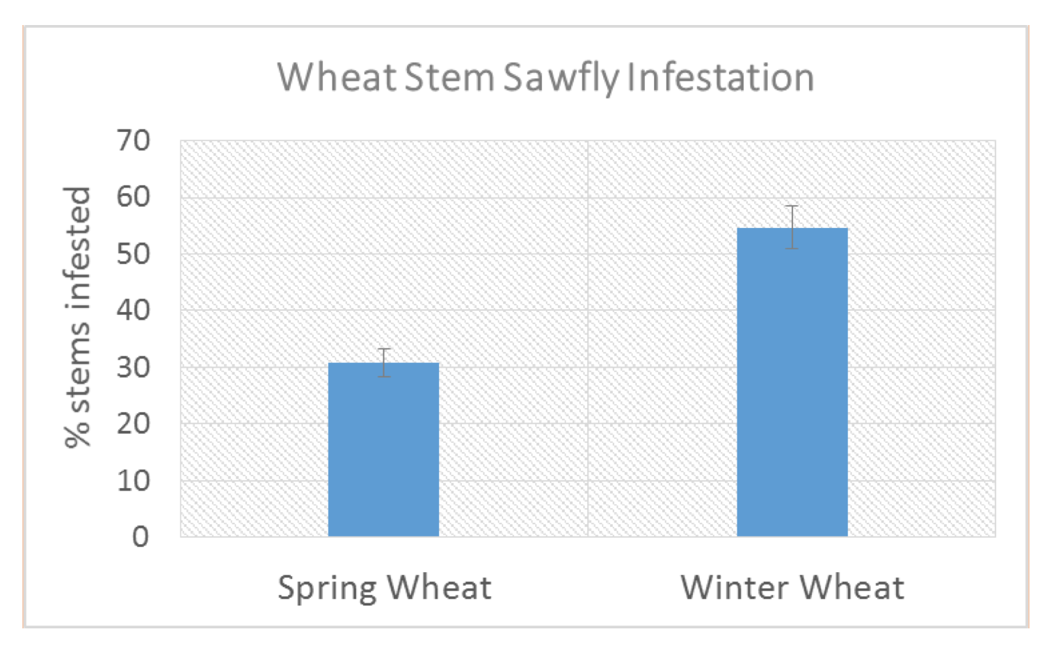 |
| Figure A5-3.1: Wheat stem sawfly infestation (± SE) in Montana wheat fields 2002 – 2016. Data from 114 spring wheat fields and 55 winter wheat fields. |
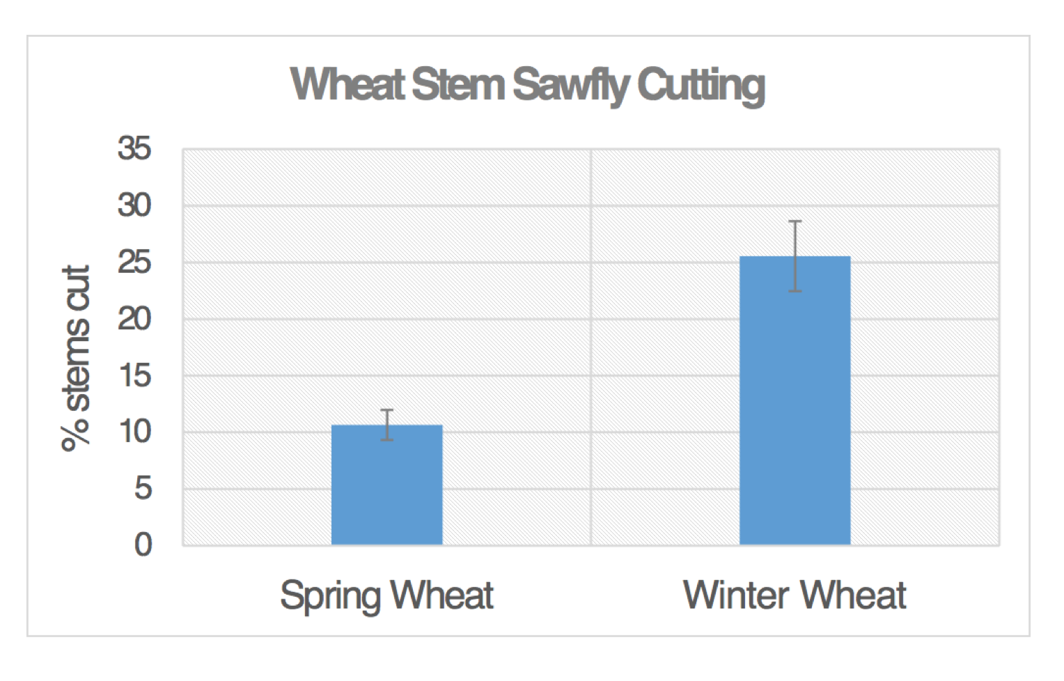 |
| Figure A5-3.2: Wheat stem sawfly stem cutting (± SE) in Montana wheat fields 2002 – 2016. Data from 114 spring wheat fields and 55 winter wheat fields. |
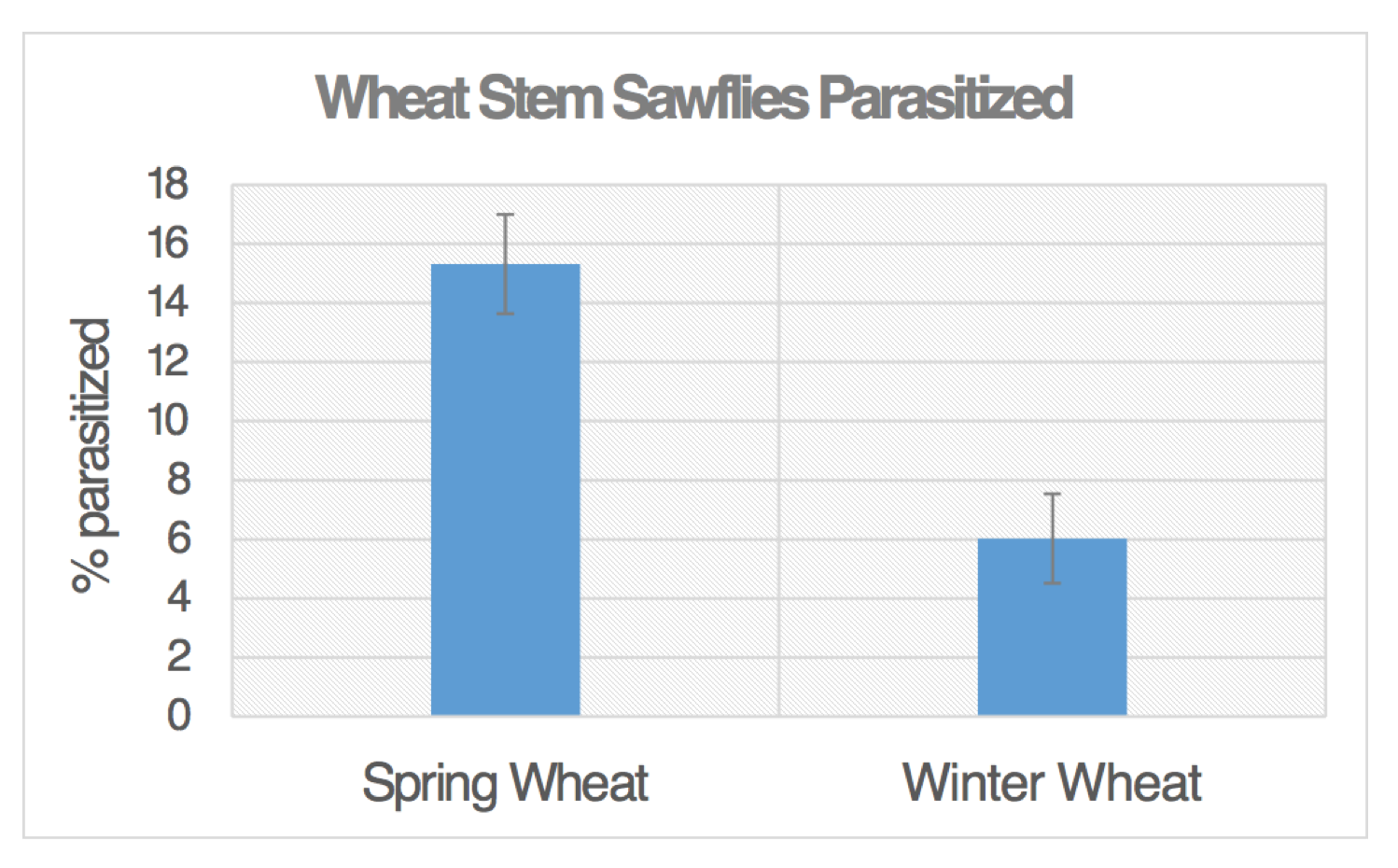 |
| Figure A5-3.3: Wheat stem sawfly larvae parasitized (± SE) in Montana wheat fields 2002 – 2016. Data from 114 spring wheat fields and 55 winter wheat fields. |
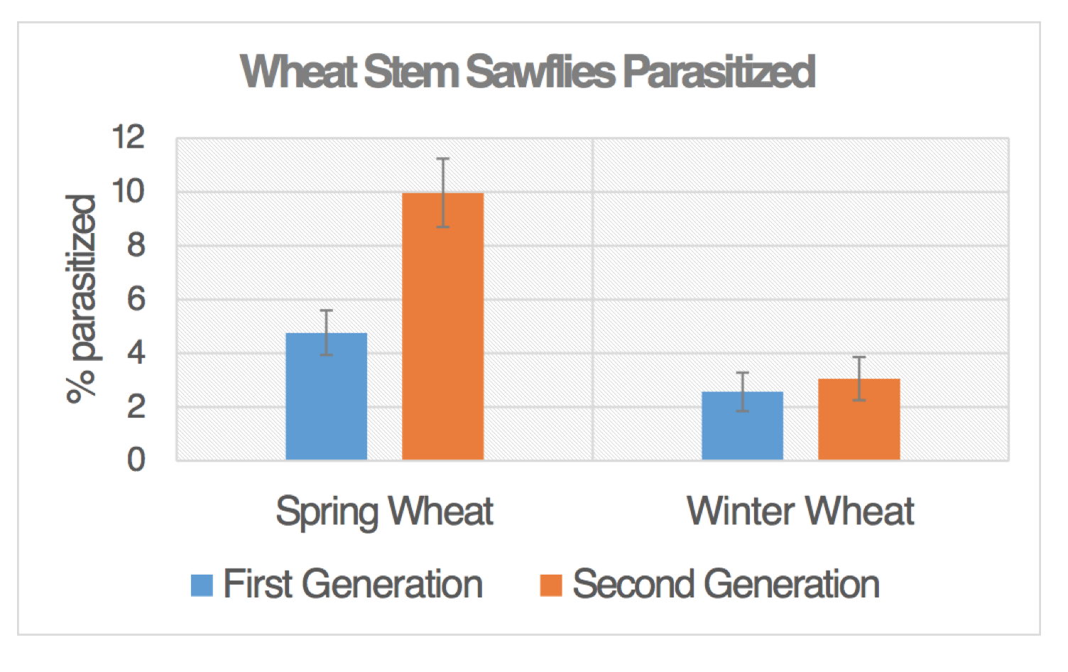 |
| Figure A5-3.4: Wheat stem sawfly larvae parasitized by 1st and 2nd generation braconids (± SE) in Montana wheat fields 2002 – 2016. Data from 111 spring wheat fields and 55 winter wheat fields. |
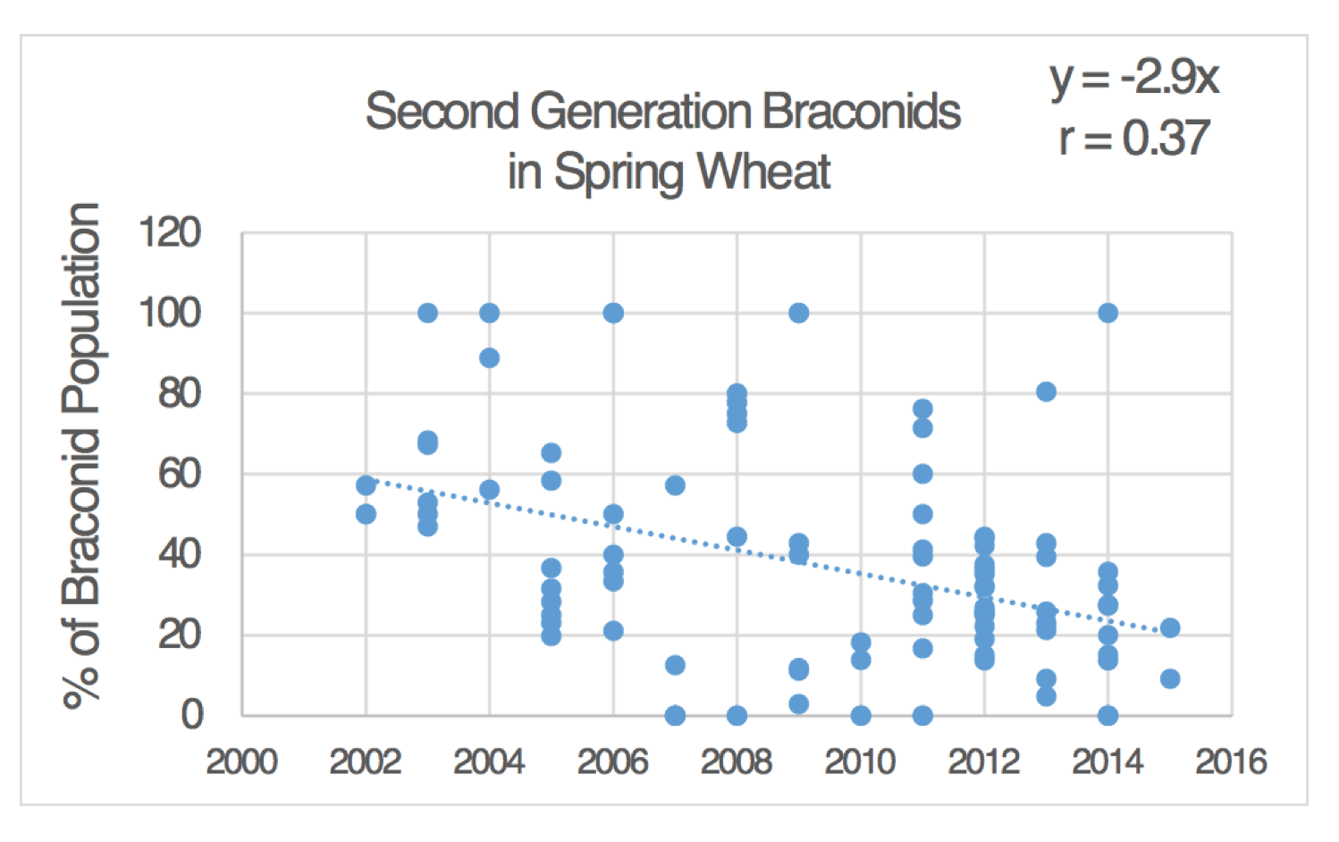 |
| Figure A5-3.5: Percentage of 2nd generation braconids as a proportion of the total braconid populations (± SE) in Montana spring wheat fields 2002 – 2016. Data from 101 fields. |
|
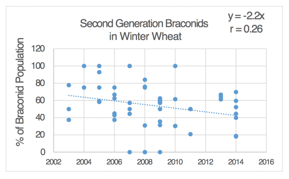
|
| Figure A5-3.6: Percentage of 2nd generation braconids as a proportion of the total braconid populations (± SE) in Montana spring wheat fields 2002 – 2016. Data from 55 fields. |
Literature Cited
Bekkerman A. 2014. Economic impacts of the wheat stem sawfly and an assessment of risk management strategies. A report to Montana Grains Foundation. Great Falls MT. 53 p. Available online http://antonbekkerman.com/docs/sawfly_economics_final.pdf. Accessed 2017 September 18.