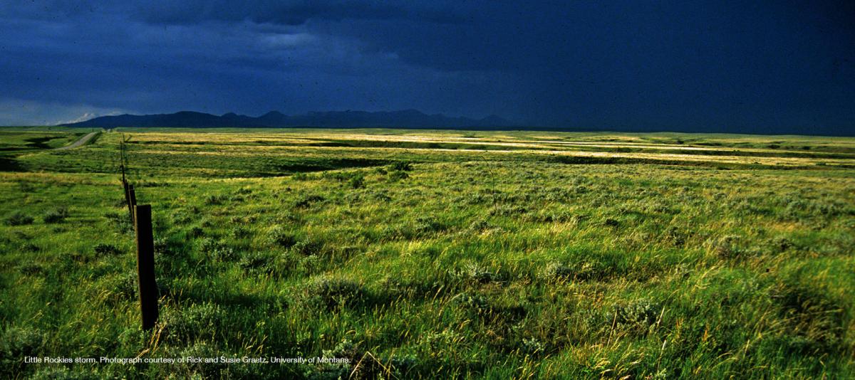
CHAPTER 2
CLIMATE CHANGE IN MONTANA
Nick Silverman, Kelsey Jencso, Paul Herendeen, Alisa Royem, Mike Sweet, and Colin Brust
Understanding current climate change and projecting future climate trends are of vital importance–both for our economy and our well-being. It is our goal to provide science-based information that serves as a resource for Montanans who are interested in understanding Montana’s climate and its impacts on water, agricultural lands and forests. To provide this understanding, we can learn from past climate trends. However, knowledge of the past is only partially sufficient in preparing for a future defined by unprecedented levels of greenhouse gases in the atmosphere. Therefore, we also provide projections of change into the future using today’s best scientific information and modeling techniques.
KEY MESSAGESAnnual average temperatures, including daily minimums, maximums, and averages, have risen across the state between 1950 and 2015. The increases range between 2.0-3.0°F (1.1-1.7°C) during this period. [high agreement, robust evidence] Winter and spring in Montana have experienced the most warming. Average temperatures during these seasons have risen by 3.9°F (2.2°C) between 1950 and 2015. [high agreement, robust evidence] Montana’s growing season length is increasing due to the earlier onset of spring and more extended summers; we are also experiencing more warm days and fewer cool nights. From 1951-2010, the growing season increased by 12 days. In addition, the annual number of warm days has increased by 2.0% and the annual number of cool nights has decreased by 4.6% over this period. [high agreement, robust evidence] Despite no historical changes in average annual precipitation between 1950 and 2015, there have been changes in average seasonal precipitation over the same period. Average winter precipitation has decreased by 0.9 inches (2.3 cm), which can mostly be attributed to natural variability and an increase in El Niño events, especially in the western and central parts of the state. A significant increase in spring precipitation (1.3-2.0 inches [3.3-5.1 cm]) has also occurred during this period for the eastern portion of the state. [moderate agreement, robust evidence] The state of Montana is projected to continue to warm in all geographic locations, seasons, and under all emission scenarios throughout the 21st century. By mid century, Montana temperatures are projected to increase by approximately 4.5-6.0°F (2.5-3.3°C) depending on the emission scenario. By the end-of-century, Montana temperatures are projected to increase 5.6-9.8°F (3.1-5.4°C) depending on the emission scenario. These state-level changes are larger than the average changes projected globally and nationally. [high agreement, robust evidence] The number of days in a year when daily temperature exceeds 90°F (32°C) and the number of frost-free days are expected to increase across the state and in both emission scenarios studied. Increases in the number of days above 90°F (32°C) are expected to be greatest in the eastern part of the state. Increases in the number of frost-free days are expected to be greatest in the western part of the state. [high agreement, robust evidence] Across the state, precipitation is projected to increase in winter, spring, and fall; precipitation is projected to decrease in summer. The largest increases are expected to occur during spring in the southern part of the state. The largest decreases are expected to occur during summer in the central and southern parts of the state. [moderate agreement, moderate evidence] |
||
Climate Change Defined
The US Global Change Research Program (USGCRP undated) defines climate change as follows: “Changes in average weather conditions that persist over multiple decades or longer. Climate change encompasses both increases and decreases in temperature, as well as shifts in precipitation, changing risk of certain types of severe weather events, and changes to other features of the climate system.”
This chapter focuses on three areas:
- providing a baseline summary of climate and climate change for Montana—with a focus on changes in temperature, precipitation, and extreme events—including reviewing the fundamentals of climate change science;
- reviewing historical trends in Montana’s climate, and what those trends reveal about how our climate has changed in the past century, changes that are potentially attributable to world-wide increases in greenhouse gases; and
- considering what today’s best available climate models project regarding Montana’s future, and how certain we can be in those projections.
This chapter serves as a foundation for the Montana Climate Assessment, providing information on present-day climate and climate terminology, past climate trends, and future climate projections. This foundation then serves as the basis for analyzing three key sectors of Montana—water, forests, and agriculture—considered in the other chapters of this assessment. In the sections below, we introduce the climate science and discuss important fundamental processes that determine whether climate remains constant or changes.
NATURAL AND HUMAN CAUSES OF CLIMATE CHANGE
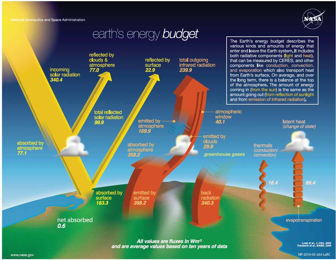
Climate is driven largely by radiation from the sun. Incoming solar radiation may be reflected, absorbed by land surface and water bodies, transformed (as in photosynthesis), or emitted from the land surface as longwave radiation. Each of these processes influences climate through changes to temperature, winds, the water cycle, and more. The overall process is best understood by considering the Earth’s energy budget (see sidebar).
|
The Earth’s Energy Budget The Earth’s climate is driven by the sun. The balance between incoming and outgoing radiation—Earth’s radiation or energy budget—determines the energy available for changes in temperature, precipitation, and winds and, hence, influences atmospheric chemistry and the hydrologic cycle. The Earth’s surface, atmosphere, and clouds absorb a portion of incoming solar radiation, thereby increasing temperatures. Energy as longwave radiation (heat) is re-emitted to the atmosphere, clouds, or space, thereby reducing temperatures at the source. If the absorbed solar radiation and emitted heat are in balance, the Earth’s temperature remains constant.
The Earth’s radiation balance is the main driver of our climate. Image courtesy of National Aeronautics and Space Administration (NASA undated).
|
Natural factors contributing to past climate change are well documented and include changes in atmospheric chemistry, ocean circulation patterns, solar radiation intensity, snow and ice cover, Earth’s orbital cycle around the sun, continental position, and volcanic eruptions. While these natural factors are linked to past climate change, they are also incorporated in the analysis of current climate change.
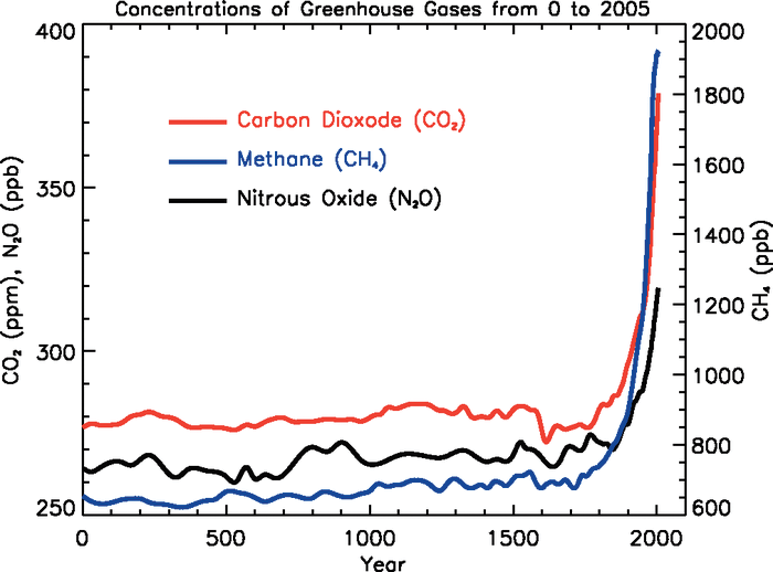
Since the Industrial Revolution, global climate has changed faster than at any other time in Earth’s history (Mann et al. 1999). This rapid rate of change—often referred to as human-caused climate change—has resulted from changes in atmospheric chemistry, specifically increases in greenhouse gases due to increased combustion of fossil fuels, land-use change (e.g., deforestation), and fertilizer production (Figure 2-1) (Forster et al. 2007). The primary greenhouse gases in the Earth’s atmosphere are carbon dioxide (CO2), methane (CH4), nitrous oxide (N2O), water vapor (H2O), and ozone (O3).
|
|
| Figure 2-1. Changes in important global atmospheric greenhouse gas concentrations from year 0 to 2005 AD (ppm, ppb = parts per million and parts per billion, respectively) (Forster et al. 2007). |
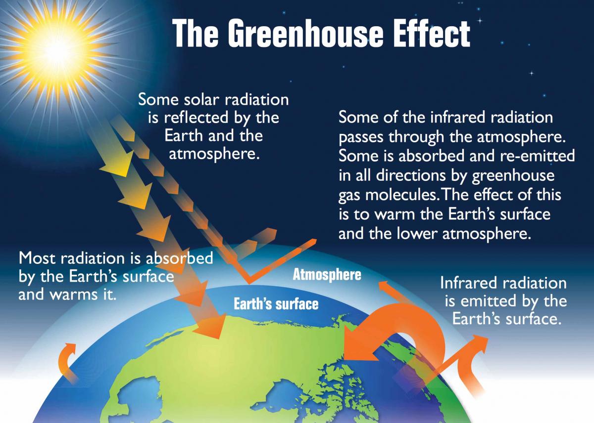
Incoming solar radiation is either absorbed, reflected, or re-radiated from the Earth’s surface. Since greenhouse gas concentrations are greatest near the surface, a large fraction of this reflected and re-radiated energy is absorbed in the lower portions of the atmosphere (hence the increase in surface temperatures and the term “greenhouse effect”—see sidebar). For the total energy budget to balance, the energy (and temperature) at the top of the atmosphere must decrease to account for the increase of energy (and temperature) near the Earth’s surface.
At natural levels, greenhouse gases are crucial for life on Earth; they help keep average global temperatures above freezing and at levels that sustain plant and animal life. However, at the increased levels seen since the Industrial Revolution (roughly 275 ppm then, 400 ppm now; Figure 2-1), greenhouse gases are contributing to the rapid rise of our global average temperatures by trapping more heat, often referred to as human-caused climate change. In the following chapters, we will refer to the impacts and effects of climate change as a result of both natural variability and human-caused climate change.
|
The Greenhouse Effect The Earth’s climate is driven by the sun. The high temperature of the sun results in the emission of high energy, shortwave radiation. About 31% of the shortwave radiation from the sun is reflected back to space by clouds, air molecules, dust, and lighter colored surfaces on the earth. Another 20% of the shortwave radiation is absorbed by ozone in the upper atmosphere and by clouds and water vapor in the lower atmosphere. The remaining 49% is transmitted through the atmosphere to the land surfaces and oceans and is absorbed. The Earth’s surface re-emits about 79% of the absorbed energy as longwave radiation. Unlike shortwave radiation, the Earth’s atmosphere absorbs approximately 90% of the longwave radiation emitted from objects on its surface. This results because of the presence of gases such as water vapor, carbon dioxide (CO2), methane (CH4), nitrous oxide (N2O), and various industrial products (e.g. chlorofluorocarbons; CFCs) that more effectively absorb longwave radiation. In turn, the energy absorbed by these gases is reradiated in all directions. The portion that is redirected back towards the surface contributes to warming and a phenomenon known as the greenhouse effect.
Climate change occurs when the Earth’s energy budget is not in balance. Such change generally takes place over centuries and millennia. Human-caused climate change has been occurring over the last 200 yr, largely because of the combustion of fossil fuels and subsequent increase of atmospheric CO2. Carbon dioxide, as well as CH4 and other gases, absorb and re-emit longwave radiation back to the earth’s surface that would otherwise radiate rapidly into outer space, thus warming the Earth. This increase in incoming longwave radiation is the greenhouse effect. Image courtesy the National Academies of Sciences (NAS undated). |
||
CLIMATE CHANGE ASSESSMENTS
A growing awareness of our changing global climate since the 1950s has led to a substantial body of research. For example, the National Academy of Sciences (NAS 2011) report, American’s Climate Choices, stated:
Climate change is occurring, is very likely caused primarily by human activities, and poses significant risks to humans and the environment. These risks indicate a pressing need for substantial action to limit the magnitude of climate change and to prepare for adapting to its impacts.
In 1990, the United Nations tasked the Intergovernmental Panel on Climate Change (IPCC, see sidebar) with assessing existing research on climate change. Since then, five IPCC assessments have increased our scientific understanding of, and certainty about, global climate change. As described later in this chapter, the assessments have incorporated increasingly sophisticated models and analyses that consider both natural and human contributions to changes in our climate system.
In its most recent Fifth Assessment Report, the IPCC raised the likelihood of changes in several global climate events to “virtually certain” (i.e., 99-100% likelihood). Examples of these events include: more frequent hot days, less frequent cold days, reductions in permafrost, and sea-level rise (IPCC 2014).
|
What is the IPCC? The Intergovernmental Panel on Climate Change is the leading international body for the assessment of climate change. It was established in 1988 by the United Nations Environment Programme and the World Meteorological Organization, and subsequently endorsed by the United Nations General Assembly. The goal of the IPCC is to provide the world with a clear scientific view on the current state of knowledge in climate change and its potential environmental and socioeconomic impacts.
|
||
Recently, the third National Climate Assessment, produced in collaboration with the US Global Change Research Program, provided further insight into the anticipated climate changes for the conterminous US. The National Climate Assessment (NCA 2014) states:
Evidence for changes in Earth’s climate can be found from the top of the atmosphere to the depths of the oceans. Researchers from around the world have compiled this evidence using satellites, weather balloons, thermometers at surface stations, and many other types of observing systems that monitor the Earth’s weather and climate. The sum total of this evidence tells an unambiguous story: the planet is warming.
MONTANA’S OBSERVED CLIMATE
To put future Montana climate change in perspective, we must first understand Montana’s baseline (i.e., historical) conditions. In this section, we describe our state’s unique geography and topography, as well as current climatology and the historical climate trends that have led us to the present day.
Geography and topography
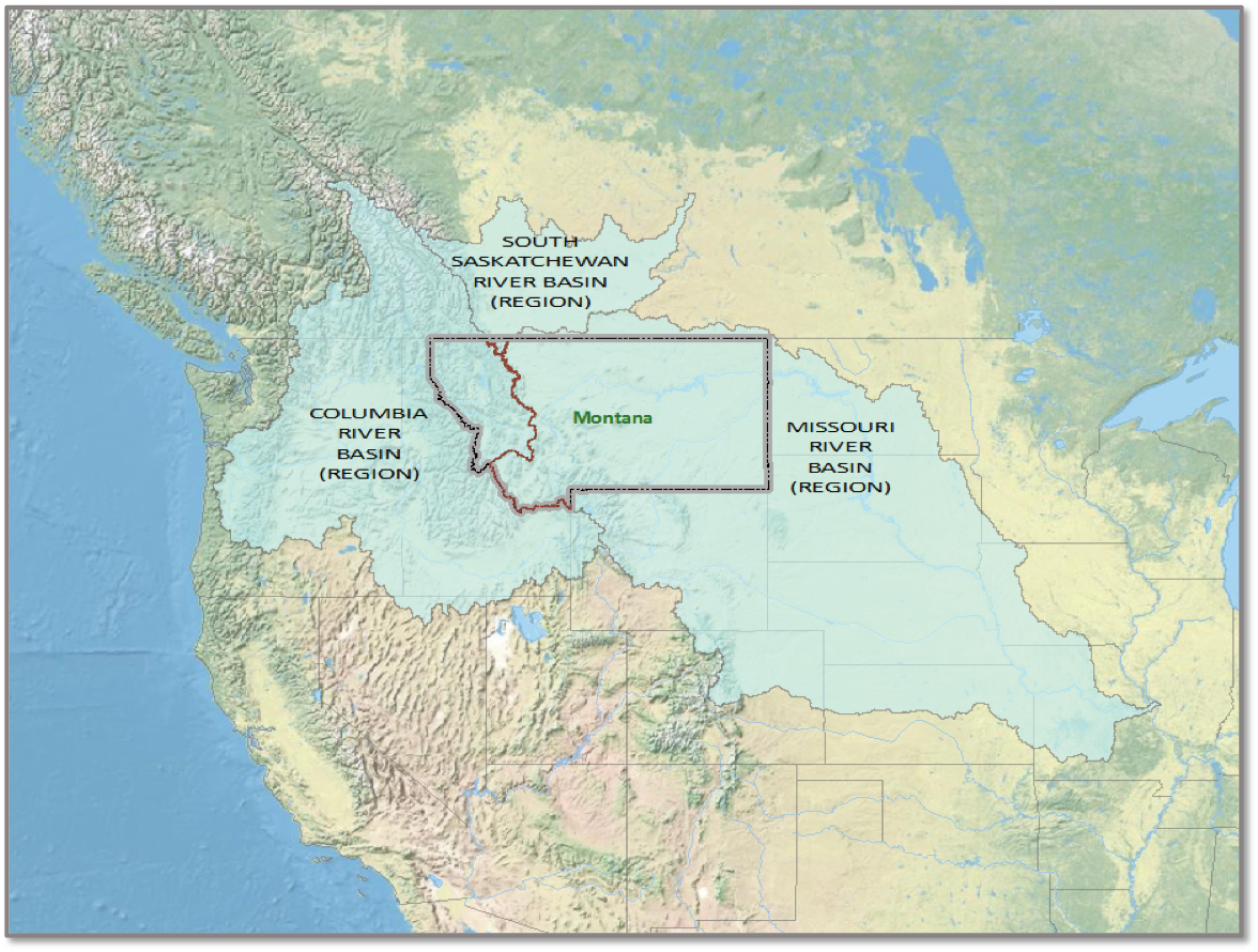
Montana is the fourth largest state in the nation, with a land area that covers 147,164 mile2 (381,153km2). The state includes the beginnings of three major river basins. Two of these—the basins of the Columbia and the Missouri rivers—encompass almost 1/3 of the landmass of the conterminous United States (Figure 2-2). Consequently, Montana’s climate influences the water supply for a large portion of the country, and its water supports tourism, agriculture, and ecosystems far beyond its borders. These attributes contribute to Montana’s reputation as the premiere headwaters state and as “The Last Best Place.”
|
|
| Figure 2-2. Montana is the fourth largest state in the nation and provides the headwaters for three major river basins. Two of these, the Columbia and the Missouri, encompass almost 1/3 of the landmass of the conterminous US. The Continental Divide is the line running through the state, and forming the Montana/Idaho border until reaching Wyoming. |
Montana’s complex geography and topography contribute to a diverse climate. The state extends from below the 45th up to the 49th parallel. Given this (relatively) high latitude, Montana receives less energy from the sun and experiences cooler temperatures than many other areas of the US. Additionally, Montana’s latitude and location within North America expose the state to a mix of diverse weather systems that commonly originate either from the Pacific Ocean or the Arctic, and sometimes from subtropical regions.
Topographically, the state’s diverse mountain and prairie landscapes (approximately 40 and 60% of the area, respectively) include elevations that range from over 12,000 ft (3660 m) in southern Montana to 1800 ft (550 m) in eastern Montana. A number of island mountain ranges also occur in the plains east of the Continental Divide amid the vast prairie landscape.
The western portion of Montana contains approximately 100 named mountain ranges that form the Rocky Mountain Continental Divide. The Continental Divide (Figure 2-2) effectively splits the state into climatically distinct western and eastern regions. The Continental Divide squeezes out moisture from eastward flowing Pacific Maritime air, creating wet and dry halves to the state. The Continental Divide runs approximately north to south, from the Canadian border to the Idaho/Wyoming border.
The mountainous area west of the Continental Divide has a climate similar to the maritime climates of the interior Pacific Northwest, with milder winters, cooler summers, and more year-round precipitation. Inversions, low clouds, and fog often form in valleys west of the Continental Divide. East of the Continental Divide, the prairie landscapes experience a semi-arid continental climate, with warmer summers, colder winters, and less precipitation.
Climate divisions
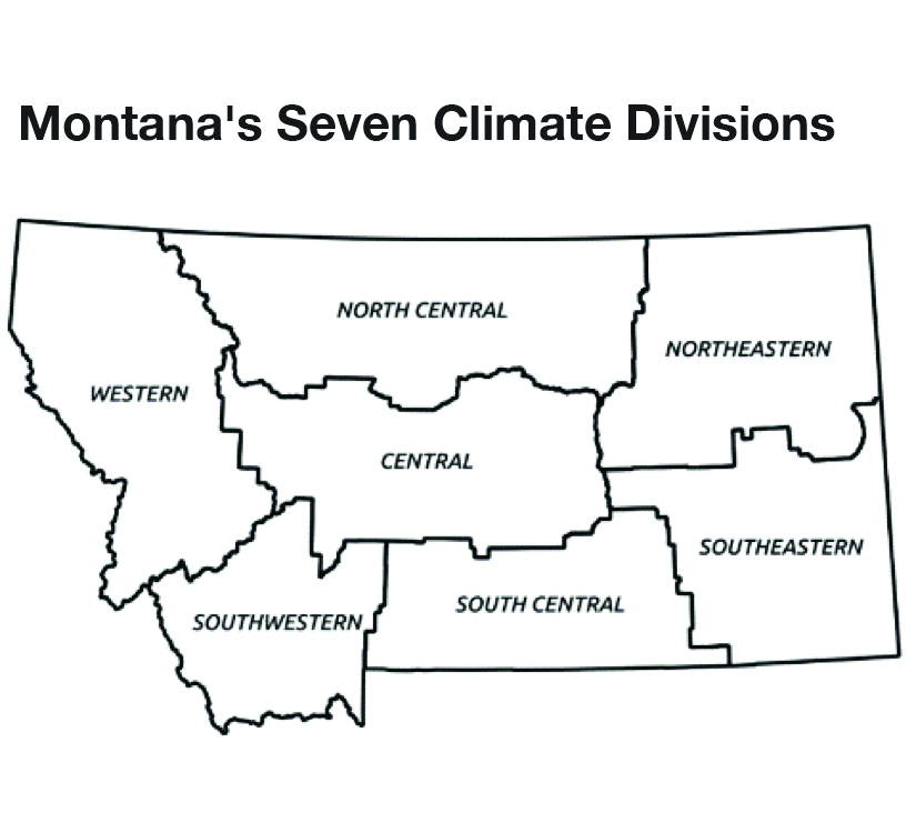
Montana’s unique geography means climate varies across the state, as it does across the nation. Thus, throughout this Montana Climate Assessment, we aggregate past climate trends and future climate projections into seven Montana climate divisions, as shown in Figure 2-3. These seven climate divisions are a subset of the 344 divisions defined by the National Oceanic and Atmospheric Administration (NOAA) based on a combination of climatic, political, agricultural, and watershed boundaries (NOAAa undated). The history of the US Climate Divisions takes many twists and turns; it is well documented in Guttman and Quayle (1996).
|
|
| Figure 2-3. Montana’s seven climate divisions. |
Current climate conditions 1981-2010
To assess Montana’s current climate, we analyzed climate variable data (see sidebar) provided as 3-decade averages by NOAA’s National Centers for Environmental Information (NOAAb undated). In this section, we review average temperature and precipitation conditions from 1981-2010 as an indicator of current climate conditions.5 In the next section on historical trends, we discuss changes in Montana’s temperature, precipitation, and extreme events that have occurred over a longer time horizon.
|
Climate Variables In analyses of climate, scientists employ a suite of 50 essential climate variables to unify discussions (Global Climate Observing System undated). For this assessment, we primarily focus on just two: how climate change will affect Montana’s temperature and precipitation in the future.
Temperature is an objective measure of how hot or cold and object is with reference to some standard value. Temperature differences across the Earth result primarily from regional differences in absorbed solar radiation. Seasonal variations in temperature result from the tilt of the Earth’s axis as it rotates around the sun.
Precipitation is the quantity of water (solid or liquid) falling to the Earth’s surface at a specific place during a given period. Like temperature, precipitation varies seasonally and from place to place. Precipitation amounts can have a dramatic impact on local environmental conditions, such as abundance of wildlife or potential for crop production.
|
||

Temperature.—Table 2-1 shows the average seasonal temperature variation across Montana’s seven climate divisions (Figure 2-3) from 1981-2010. Temperatures vary widely across Montana and are strongly dependent on local elevation and proximity to the Continental Divide. Western Montana’s annual average temperatures are generally cooler (approximately 39°F [3.9°C]) relative to the eastern and central parts of the state (approximately 44°F [6.7°C]).
| Montana climate division | Annual | Winter (avg / avg minimum) | Spring | Summer (avg / avg maximum) | Fall |
| Northwestern | 40.6 | 23.7 / 16.5 | 39.4 | 58.5 / 72.0 | 40.6 |
| Southwestern | 38.9 | 21.2 /12.4 | 37.3 | 57.5 / 71.5 | 39.4 |
| North central | 42.8 | 21.8 / 10.9 | 42.1 | 63.8 / 78.3 | 43.1 |
| Central | 43.3 | 24.8 / 14.6 | 41.8 | 62.7 / 77.1 | 43.5 |
| South central | 44.0 | 24.6 / 14.2 | 42.5 | 64.3 / 78.8 | 44.2 |
| Northeastern | 43.4 | 18.3 / 7.9 | 43.3 | 67.4 / 81.6 | 44.0 |
| Southeastern | 45.5 | 22.8 / 11.7 | 44.6 | 68.6 / 83.2 | 45.8 |
Winters in Montana are cold, with statewide average temperatures of 22°F (-5.6°C). Between cold waves there are often periods of mild, windy weather in central Montana created by persistent, moist Pacific air masses on the west side of the Continental Divide, and the drying and warming effects as air descends on the east side of the Rockies. These surface winds are locally known as chinook winds and can bring rapid temperature increases of 40-50°F (22-28°C) to areas east of the Rockies that can last for days.
Montana springs are highly variable and bring dramatic temperature changes. As a whole, Montana’s average spring temperature is 42°F (5.5°C), although western Montana is cooler and warming comes later due to persistence of Pacific maritime air. In contrast, warmer continental air contributes to average temperatures up to 45°F (7.2°C) in spring across central and eastern Montana.
Elevation and proximity to the Continental Divide strongly influence local temperatures in summer. Valleys and the eastern plains are generally warmer than the higher elevations of the Continental Divide. While summer average temperature across Montana is 64°F (17.8°C), temperatures generally peak in
July and August, with mean daily highs above 90°F (32°C) in the east, as well as in western valleys.
Fall temperatures in Montana are often highly variable, with an average temperature of 43°F (6.1°C). Days to weeks of warm temperatures are commonly followed by freezing temperatures that bring frosts and snow.
Precipitation.—In general, Montana is a water-limited, semi-arid landscape where precipitation is depended upon heavily by plants and animals alike. Table 2-2 shows the seasonal variation of precipitation across Montana’s seven climate divisions (Figure 2-3) from 1981-2010. Precipitation amounts and form (rain versus snow) vary widely across the state and are strongly influenced by elevation and proximity to the Continental Divide. The average annual precipitation for Montana is 18.7 inches (0.47 m). Western Montana typically receives twice as much precipitation annually as eastern Montana (22-30 inches [0.56-0.76 m] versus 12-14 inches [0.30-0.36 m], respectively). The combination of moisture-rich maritime air from the Pacific in the winter, spring, and fall, and strong convective systems in the summer create a more evenly distributed year-round precipitation pattern in western Montana. In contrast, 65-75% of the annual precipitation occurs in the late spring and summer months for eastern and central Montana, coming from sources in the subtropical Pacific and Gulf of Mexico.
| Montana climate division | Annual | Winter (avg / avg minimum) | Spring | Summer (avg / avg maximum) | Fall |
| Northwestern | 32.4 (82.2) | 9.4 (23.9) | 8.9 (22.6) | 6.1 (15.5) | 8.1 (20.6) |
| Southwestern | 21.2 (53.8) | 4.1 (10.4) | 7.1 (18.0) | 5.5 (14.0) | 4.6 (11.7) |
| North central | 15.1 (38.4) | 1.9 (4.8) | 4.6 (11.7) | 5.5 (14.0) | 3.1 (7.9) |
| Central | 17.6 (44.7) | 2.4 (6.1) | 5.8 (14.7) | 5.9 (15.0) | 3.5 (8.9) |
| South central | 18.4 (46.7) | 2.7 (6.9) | 6.4 (16.3) | 5.2 (13.2) | 4.2 (10.7) |
| Northeastern | 12.8 (32.5) | 1.0 (2.5) | 3.7 (9.4) | 5.7 (14.5) | 2.4 (6.1) |
| Southeastern | 13.8 (35.1) | 1.2 (3.0) | 4.6 (11.7) | 5.1 (13.0) | 2.9 (7.4) |
The average statewide precipitation during winter is 3.3 inches (8.4 cm), though it varies considerably across the state. The majority of winter precipitation in Montana falls as snow, and the precipitation that accumulates as snowpack in the mountains is the most significant source of water to valley bottoms throughout the summer. Northwestern Montana receives an average of 9.4 inches (23.9 cm) of winter precipitation, but locally, and at higher elevations within the mountains, this value can increase to greater than 20 inches (50.8 cm). Eastern and central Montana typically receive 1.0-2.7 inches (2.5-6.9 cm) of winter precipitation.
Montana receives significant spring precipitation, with a statewide average of 5.8 inches (14.7 cm). Much of that precipitation contributes to the recharge of shallow soil moisture and groundwater supplies. This storage plays an important part in Montana’s water cycle by releasing water slowly throughout the summer. Spring precipitation averages range from 7-9 inches (17.8-22.9 cm) in the west to 3-6 inches (7.6-15.2 cm) for prairie lands of central and eastern Montana.
The average summer precipitation for Montana, which is relatively consistent statewide, is 5.6 inches (14.2 cm). Convective thunderstorms are responsible for most of the summer precipitation across the state. These storms result from the uplift of warm, moisture-laden air masses originating from the subtropical Pacific and Atlantic. As the air rises, it cools and water vapor condenses, producing rainfall and, at times, large amounts of damaging hail.
The average fall precipitation for Montana is 4.1 inches (10.4 cm). Northwestern Montana experiences the largest average amount of precipitation (8.1 inches [20.6 cm]). Average fall precipitation declines as one moves to central and then eastern Montana (approximately 3.6 and 2.7 inches [9.1 and 6.9 cm], respectively).
Historical trends 1950 to present
We evaluated how temperature and precipitation have historically changed, dating back to mid-20th century. This review of historical trends helps us provide context for future climate change scenarios explored in later sections of this chapter. In addition, evaluating these trends can help us better understand a) how Montanans have previously experienced and responded to changing climate, b) if projections of future change reveal a different climate than we have previously experienced, and c) the potential impacts of that projected change.
We used standard statistical methods to analyze records of temperature and precipitation spanning two periods: 1950–2015 and 1900–2015.6 The direction (increase or decrease) and significance of trends were generally similar for the two periods. As such, the presentation of trends that follows is confined to the period from 1950–2015. This is widely acknowledged as the benchmark period in climate analysis (Liebmann et al. 2010; IPCC 2013a), a period when our network of meteorological sensors becomes more accurate and sufficiently dense. It also coincides with an upward inflection of the annual average temperature trend for Montana, demarcating a time period with the highest rate of change and likely the strongest anthropogenic signal (NOAAc undated).
Our analysis uses observational data from the US Climate Divisional Database (NOAAc undated) to provide a more complete picture. The data were corrected to remove observational bias (e.g., station relocation, instrumentation changes, and observer practice changes) (Vose et al. 2014). Our approach included combining many stations to provide a more complete picture of historical changes for large regions. In our analyses, we determined if a detectable trend existed for temperature and/or precipitation across the seven climate divisions and/or the entire state. While not included in our analysis, other sources of historical climate data such as local observation are also extremely valuable to confirm measured trends and their impacts (see sidebar).
|
Crow Climate Observations John Doyle and Margaret Eggers As the Crow Environmental Health Steering Committee, a group of Crow Tribal stakeholders working on local water quality and health issues, we began discussing long-term changes in local climate and ecosystems we’ve observed in our lifetimes. This began a process of interviewing other Tribal members on this topic, and then comparing our community knowledge to climate and hydrological data available for the Crow Reservation and vicinity. We found that these two sources of data correspond and complement one another, with our observational data filling in gaps where no monitoring sites exist, and providing information on impacts to local foods, cultural traditions, and community health. There is widespread agreement among Tribal Elders interviewed that winter snowfall is declining, winters are getting milder and summers are becoming hotter. The prairies used to be covered in deep snow from November to March, often making it difficult to feed livestock; the rivers would freeze up and as kids we could ice skate all winter long, including along the rivers. With winter, the wind would shift to come primarily from the north, instead of from the west—a sign to us that winter had come. Now the prairies are commonly barren of snow, rivers have thin ice if at all, and there are successive winter days above freezing when the trees thaw out, only to be damaged when freezing conditions return. Sometimes a winter snowfall turns into rain, which never used to happen. It’s hard to predict the winter weather anymore, as we once could in the old days. These changes also seem to affect community health: The long winter cold was associated with less illness; we associate the increasing incidence of colds and flu with milder winters. Around March, ice breakup on the river used to be a major event, scouring the riverbeds and leaving large chunks of ice to slowly melt on the riverbanks. This was accompanied by a traditional Crow ceremony. By April, the snow would be gone and brooks would be running everywhere. Now the thin ice simply melts away quietly, and the ephemeral brooks don’t all flow. We would get storms when it would rain really hard for 10-15 minutes, now the spring storms come with severe winds and sleet or hail. However, spring flood events are more frequent now. Before the flood in the 1970s and the two severe floods in the past decade, the only one our parents remember was in 1921. Summer heat lasts longer than it used to, and is more intense. We used to get summer rains that broke the heat, now that hardly happens anymore; when it stays hot for a long time, it seems to affect the vegetation. Plants are a good way of finding out the weather: when their leaves don’t grow to their fullest, we know the weather, the climate, is changing. Boxelder trees and some of the berry shrubs along the river are slowly dying. Riparian berries, including plums, chokecherries, juneberries, and buffalo berries, have been gathered for generations as staple foods. Sometimes they now bloom earlier in the spring; cold snaps freeze the blossoms and the berry crops are lost. Sundances—a traditional outdoor ceremony in which both men and women dance, pray and fast without either food or water for 3 to 4 days—have always been held in the same locations in May and June. People who have sundanced over many years say it is becoming more difficult, as these months are increasingly hotter and drier. One Elder remarked that there were never any bad forest fires when he was a boy; those fires didn’t start until the 1950s. The disappearance of some insect species, the flocking of birds, animals growing thicker coats, and snow on the mountains were always signs of winter—it is now mid-November, still T-shirt weather with no snow on the mountains, and the grasshoppers and most summer birds are still around. We used to gather buffalo berries in the fall after the first frost sweetened the berries; now the first frost doesn’t come before the berries dry up, so they aren’t worth harvesting. There are a lot of species which are no longer here or are rarely seen—perhaps due to climate changes, perhaps population. Barn owls, burrowing owls, snipes, certain hawks, prairie chickens, and blue grouse are gone. Kangaroo mice and another mouse that was always nesting used to be common. Frogs used to croak all night long in the summers, now you don’t hear them anymore. Small turtles, freshwater mussels, and a riverbank lizard species have disappeared. In addition to the declining availability of berries, other food plants such as wild turnip and wild carrot, which used to be all over, have become scarce. We all see these changes, but there seems to be a reluctance to talk about what’s happening, to name it. As one Elder, G. Bulltail, concluded,
The rivers are powerful, they have energy and they make things grow. We used to go to the river to communicate with this energy, now we just go there to fish and to swim. Nature used to provide for us, and we put back what we got, but we don’t do that anymore. Everything is getting polluted—the air isn’t clean anymore. The Earth is trying to tell us that we have to go back to a time when we saw the energy in Earth, when we were compatible with Nature.
Image of Little Bighorn River courtesy John Doyle. John Doyle is a Crow Tribal Elder and Water Quality Project Director at Little Big Horn College. Mari Eggers is a Research Scientist at Montana State University Bozeman. The authors would like to acknowledge and thank Urban Bear Don’t Walk, Grant Bulltail, Larry Kindness, MA LaForge, Bill Lincoln, Larson Medicine Horse, K. Red Star, David Small, Sara Young, and David Yarlott Jr for contributions to this article. Insignia provided by John Doyle and Mari Eggers with permission. |
||
Temperature.—Table 2-3 shows the decadal rate of change from 1950-2015 for average annual temperatures across Montana. We provide that rate of change both annually and by season for the seven Montana climate divisions depicted in Figure 2-3. We also present the average annual and average seasonal changes statewide and for the US as a whole. To account partially for autocorrelation we considered trends as significant with a conservative p value at p<0.05. Generally, Montana has warmed at a rate faster than the annual national average, as well as within individual seasons.
| Montana climate division | Annual | Winter (avg / avg minimum) | Spring | Summer (avg / avg maximum) | Fall |
| Northwestern | +0.39 (+0.22) | +0.38 (+0.21) | +0.49 (+0.27) | +0.38 (+0.21) | +0.29 (+0.16) |
| Southwestern | +0.35 (+0.19) | 0 (0) | +0.58 (+0.32) | +0.30 (+0.17) | +0.23 (+0.13) |
| North central | +0.51 (+0.28) | +0.85 (+0.47) | +0.62 (+0.34) | +0.30 (+0.17) | 0 (0) |
| Central | +0.43 (+0.24) | +0.59 (+0.33) | +0.59 (+0.33) | +0.29 (+0.16) | 0 (0) |
| South central | +0.44 (+0.24) | +0.49 (+0.27) | +0.61 (+0.34) | +0.36 (+0.20) | +0.30 (+0.17) |
| Northeastern | +0.48 (+0.27) | +0.78 (+0.43) | +0.65 (+0.36) | +0.26 (+0.14) | 0 (0) |
| Southeastern | +0.40 (+0.22) | +0.59 (+0.33) | +0.56 (+0.31) | 0 (0) | 0 (0) |
| Statewide | +0.42 (+0.23) | +0.56 (+0.31) | +0.40 (+0.22) | +0.30 (+0.17) | +0.25 (+0.14) |
| US | +0.26 (+0.14) | +0.30 (+0.17) | +0.40 (+0.22) | +0.18 (+0.10) | +0.18 (+0.10) |
Average annual temperatures increased for the entire state and within all climate divisions (see Figure 2-3). The rate of temperature increase was 0.4°F/decade (0.2°C/decade) across the state, and this rate was relatively constant across all climate divisions (Table 2-3). Similarly, average annual maximum and minimum temperatures increased statewide, and for all seven climate divisions, by 0.3-0.6°F/decade (0.2-0.3°C/decade). Between 1950 and 2015, Montana’s average annual temperature has increased by 2.7°F (1.5°C); annual maximum and minimum temperatures have increased approximately 3.3°F (1.8°C).
Between 1950 and 2015, average annual temperature increased for the entire state of Montana and within all climate divisions. The state average annual temperature increased 2.7°F (1.5°C); annual maximum and minimum temperatures increased approximately 3.3°F (1.8°C).
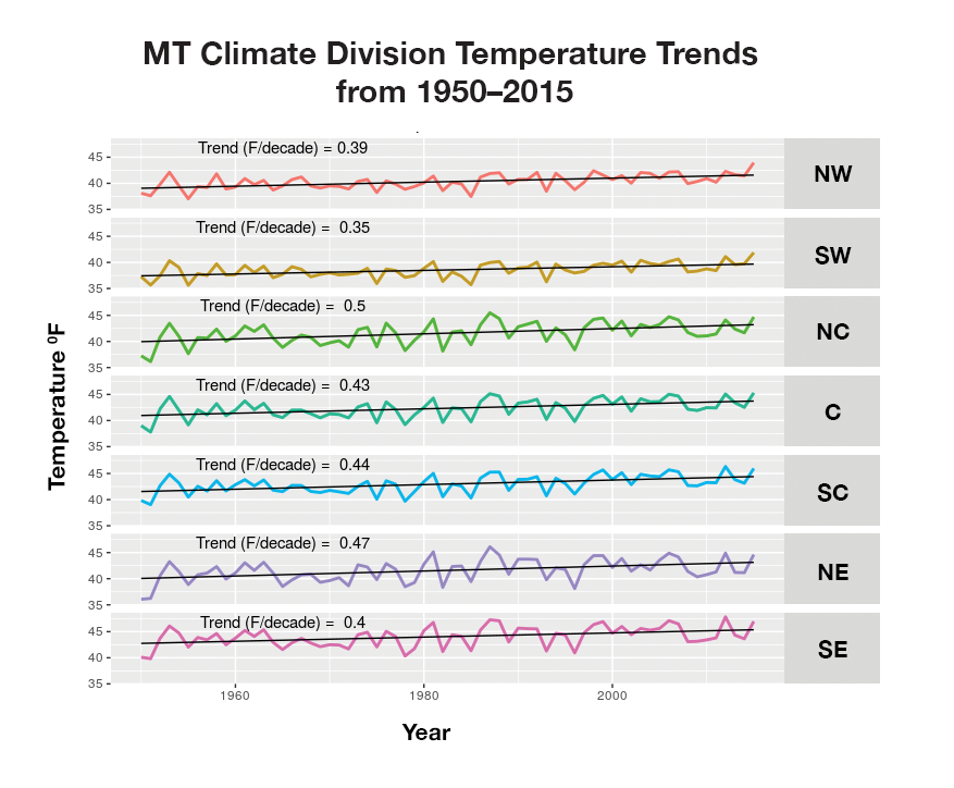
Figure 2-4. Trends in annual average temperature across each climate division (Figure I) in Montana. The divisions are northwestern (NW), southwestern (SW), north central (NC), central (C), south central (SC), northeastern (NE), and southeastern (SE).
Precipitation.—Annual precipitation averaged across the state has not changed significantly since 1950. Some change, however, has occurred within different climate divisions and for different seasons as shown in Table 2-4. We found no significant changes in summer and fall precipitation between 1950-2015 for any climate division. Seasonally, the largest changes—declines—in precipitation (rain and snow combined) have occurred during winter months (Table 2-4). We used a smaller p value (<0.05) to determine statistical significance of trends and to account for potential autocorrelation of time series data. Our analysis suggests that an increase in the number of El Niño events since 1950 has contributed to drier winters and decreased precipitation for Montana’s northwestern, north central, and central climate divisions (see Teleconnections section for more on the El Niño Southern Oscillation). In the eastern portions of the state significant increases in precipitation have occurred during the spring months (Table 2-4).
| Montana climate division | Annual | Winter (avg / avg minimum) | Spring | Summer (avg / avg maximum) | Fall |
| Northwestern | -0.58 (-1.5) | -0.57 (-1.4) | 0 | 0 | 0 |
| Southwestern | 0 | 0 | 0 | 0 | 0 |
| North central | 0 | -0.09 (-0.23) | 0 | 0 | 0 |
| Central | 0 | -0.11 (-0.28) | 0 | 0 | 0 |
| South central | 0 | 0 | 0 | 0 | 0 |
| Northeastern | 0 | 0 | +0.21 (+0.53) | 0 | 0 |
| Southeastern | +0.35 (+0.89) | 0 | +0.30 (+0.76) | 0 | 0 |
| Statewide | 0 | -0.14 (-0.36) | 0 | 0 | 0 |
| US | +0.33 (+0.84) | 0 | +0.08 (+0.20) | +0.08 (+0.20) | +0.16 (+0.41) |
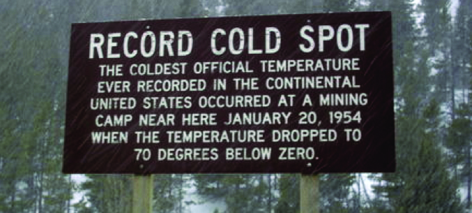
Extreme aspects of Montana’s climate.—Along with analyzing historical trends in temperature and precipitation, we performed an analysis of changes in extreme climate events since the middle of last century. Two examples of climate extremes include periods of intense warm or cool temperatures and significant wet or dry spells across seasons. Because these events affect every aspect of our society, decision makers and stakeholders are increasingly in need of historical evaluations of extreme events and how they are changing from seasons to centuries. The coldest temperature ever observed in the conterminous US was -70°F (-57°C) at Rogers Pass outside of Helena on January 20, 1954 (see sidebar). Since 1950, however, our analysis shows the average winter temperature has increased by 0.4°F/decade (0.2°C/decade) across the state, with an overall average winter temperature increase of 3.6°F (2.0°C). Average spring temperatures have increased by 2.6°F (1.4°C) during the same period, and average summer temperatures have risen by 2.0°F (1.1°C). Montana’s fall average temperatures have increased by 1.6°F (0.9°C) since 1950.
|
Rogers Pass,Montana C. Corby Dickerson IV One-half mile west of Rogers Pass and just south of the Continental Divide, a humble cabin was nestled next to a fledgling gold mine. The cabin sat within a small, “saucer-shaped depression” in the hills. It was 1954. The weather had been unrelenting: heavy, intense snow had fallen near continuously for 7 days, totaling over 5 ft (1.5 m) deep by 5 PM on the 19th of January. The temperature that morning had been a frigid -37°F (-38°C). But, unbelievably, these measurements themselves would ultimately pale in comparison to what would occur later that night. Meteorologically, conditions had been ideal for a prolonged, heavy snow event. A steady feed of relatively warm and very moist Pacific air had, for several days, rested over a comparatively dry and persistent Arctic air mass from Canada. As the sun set on the horizon, the snow ceased and the wind, which had been biting from the northeast for days, was notably weaker. After settling in for another night of trying to stay warm in his family’s primitive surroundings, official US Weather Bureau observer H.M. Kleinschmidt resolved to stay awake much of the night due to, as described by Dightman (1963), … loud and frequent “popping” noises in the cabin, and that about 2 AM on the 20th he had observed his [unofficial] thermometer (exposed outside an insulated window several inches from the building) to show about -68°F. Mr. Kleinschmidt, despite the extreme and dangerous cold, ventured outside to check the official instrument shelter where he found the minimum thermometer to read colder than -65°F (-54°C), which was as far down the scale as the government-issued thermometer could read. Later that day at observation time, he recorded the minimum temperature as -68°F (-56°C), completely unaware that this would come to set a record for the coldest reading ever taken in the United States! Thereafter, the Kleinschmidts went about their business as rugged Montana miners, while the weather gradually returned to more normal January conditions. Although this record temperature occurred on January 20th, the Weather Bureau remained unaware of it until the observation form arrived at its Helena office on February 3rd. In reviewing this data, program manager and State Climatologist R. A. Dightman immediately noted the remarkable reading. Believing it to be a potential record, Dightman contacted the observer, requesting he send in the minimum thermometer for evaluation. The Kleinschmidts had been noted as doing “very well and keep[ing] a good record”as observers (Dightman 1963). (It is standard practice to send instrumentation to the US Weather Bureau lab in Washington, DC for calibration and verification when such extreme records are possible.) Yet Kleinschmidt, the good observer he was, actually did one better and sent in both the official minimum thermometer and his personal minimum thermometer for evaluation. While in the lab, scientists recreated the extreme conditions and observed the official and unofficial thermometers just as Kleinschmidt had described: the marker floating in the official liquid thermometer retreated back into its bulb and remained stuck there, pinned at an angle against the glass. This made it impossible for an actual reading much below the scale of this thermometer. But through additional laboratory analysis, along with the verified reading on the unofficial minimum thermometer, the US Weather Bureau was able to declare the coldest temperature observed that morning as -69.7°F (-57°C). Now confirmed as a valid observation, this reading was cross-checked against additional nearby stations (which had recorded -57°F [-49°C] and -59°F [-51°C] that same day) for reasonable consistency. After passing this final test and by knowing that they were good observers who were unaware of the potentially record-breaking nature of this observation, the US Weather Bureau on March 16, 1954 accepted the -70°F (-57°C) reading as the official all-time record low for the US. Seventeen years later a reading of -79.8°F (-62°C) was observed at Prospect Creek Camp in Alaska, establishing a new record for the country. However, to this day the reading at Rogers Pass, Montana is still the coldest ever observed throughout the conterminous US—a reading that astounds as much as it reveals about the limitlessness of nature.
This highway marker near Rogers Pass commemorates the record cold of 1954. C. Corby Dickerson IV is a General Forecaster with the National Weather Service in Missoula, MT who also leads various graphical and social media programs. The author acknowledges a) Chris Gibson and Paul Fuhr for their editing assistance; and b) Matt Moorman, Michael Zenner, Dave Bernhardt, Gina Loss, and the staff at the National Centers for Environmental Information for their valuable assistance in helping track down the story behind this historic observation. |
||
We performed our analysis of climate extremes using the CLIMDEX project (CLIMDEX undated), which provides a collection of global and regional climate data from multiple sources. CLIMDEX is developed and maintained by researchers at the Climate Change Research Centre and the University of New South Wales, in collaboration with the University of Melbourne, Climate Research Division of Environment Canada, and NOAA’s National Centers for Environmental Information. The CLIMDEX project aims to produce a global dataset of standardized indices representing the extreme aspects of climate. Particular attention was placed on the changes in variables such as consecutive dry days, days of heavy precipitation, growing season length, frost days, number of cool days and nights, and the number of warm days and nights. Extreme precipitation events across the United States have increased in both intensity and frequency since 1901 (NCA 2014), including across both the High Plains and the northwestern US (many states combined), where studies have shown an increase in the number of days with extreme precipitation (NCA 2014). However, for our analysis at the state level we found no evidence of changes in extreme precipitation so it is not a variable of focus. Here, we report those variables that did change significantly (p<0.05) for Montana and, for perspective, the climate normals for these extremes for the periods 1951–1980 and from 1981-2010 (Table 2-5).7
| Variable | Change (1951-2010) | 1951–1980 | 1981–2010 |
| Warm days | 11 days | 30 days | 41 days |
| Cool days | -13 days | 43 days | 30 days |
| Frost days | -12 days | 171 days | 159 days |
| Growing season | 12 days | 194 days | 206 days |
| Warm nights | 14 nights | 30 nights | 44 nights |
| Cool nights | -12 nights | 43 nights | 31 nights |
| Monthly minimum temperature | 5°F (2.8°C) | -25°F (-32°C) | -20°F (-29°C) |
| Monthly maximum temperature | 1.1°F (0.6°C) | 97.5°F (36°C) | 98.6°F (37°C) |
The annual number of cool days and the number of days with frost are decreasing across Montana. We use the CLIMDEX definition of cool days as the percentage of days when maximum temperature is lower than 10% of the historical observations. Coincident with warming temperatures, the number of cool days each year during the period from 1951–2010 has decreased by 13.3 days. Along with this trend, the number of days in which the minimum temperatures are below 32°F (0°C; i.e. frost days) has decreased by 12 days during this time period. These trends have contributed to an overall increase in the growing season length of 12 days between 1951 and 2010. In addition, the number of warm days, where maximum temperature exceeds 90°F (32°C) based on historical conditions, has increased by 11 days over this period. At a sub-annual level, monthly maximum and minimum temperatures have also changed. These are defined as the monthly maximum (minimum) value of daily maximum (minimum) temperatures. Monthly minimum values of daily minimum temperatures have increased by 5°F (2.8°C) from the period 1951–2010. Over the same time period, monthly minimum values of daily maximum temperatures have increased by 1.1°F (0.6°C).
There has been an increase in the number of warm nights and a related decrease in the number of cool nights across Montana. We use the CLIMDEX definition of warm nights (and cool nights) as the number of days when minimum temperature is higher (lower) than a specified maximum (minimum) threshold defined by historical conditions. The number of warm nights has increased by 11 days from 1951 to 2010. The number of cool nights has decreased by 12 days over this same period. These trends are in agreement with observations across many portions of the continental US (Davy and Esau 2016).
Between 1951 and 2010, the growing season in Montana increased 12 days.
|
Drought Drought is a recurrent climate event that may vary in intensity and persistence by region. Drought can have broad and potentially devastating environmental and economic impacts (Wilhite 2000); thus, it is a topic of ongoing, statewide concern. Through time, Montana’s people, agriculture, and industry, like its ecosystems, have evolved with drought. Today, many entities across the state address drought, including private and non-profit organizations, state and federal agencies, and landowners, as well as unique watershed partnerships. Drought is a complex phenomenon driven by both climate, but also affected by human-related factors (e.g., land use, water use). Although the definition of drought varies in different operational contexts, most definitions include several interrelated components, including:
While the subsequent chapters dealing with water, agriculture, and forests treat the subject of drought differently, each describes drought within the context of one or more of the four definitions described above. |
||
Teleconnections
When we think of weather, we generally think about what is happening around us at that moment. However, the Earth’s atmosphere, oceans, and landmasses make up a continuous system, and what we experience as weather—and also in expanded time frames as climate—is actually a small part of much larger patterns of atmospheric circulation that determine movements of air, moisture, and energy across the planet. Atmospheric circulation takes on recurring patterns that link the weather and climate across distant parts of the globe. Scientists call these recurring or persistent patterns, teleconnections. Teleconnections thus are climate oscillations that link across vast geographical areas and can last for weeks to decades.
In the past, scientists identified teleconnections by observing patterns in historical climate and weather data, and then investigating the underlying processes driving those patterns. As global climate changes, the nature of these connections is changing, as well. We can no longer rely only on historical observations to understand future teleconnections. Thus, predicting climate-related changes in teleconnections and the impact of those changes on local weather and climate are important areas of ongoing research.
Scientists recognize many teleconnections. We describe two of the most important teleconnections for Montana below, the El Niño-Southern Oscillation and the Pacific Decadal Oscillation.8 It is important to bear in mind that teleconnections are happening continually, and superimposed on each other as well as upon other long-term climate patterns. As such, teleconnections may mask the trend of a longer-term climate signal or enhance the signal making it appear stronger than it is. Additionally, teleconnections can be helpful in identifying likely seasonal and annual weather patterns and, in some cases, longer-term climate trends.
El Niño-Southern Oscillation.—The El Niño-Southern Oscillation cycle refers to a fluctuation between unusually warm (El Niño) and cold (La Niña) waters in the tropical Pacific, with associated changes in atmospheric circulation (the Southern Oscillation) (Figure 2-5). El Niño and La Niña events typically develop over 2-7 yr. During El Niño events, western North America experiences greater flows of maritime air and reduced flows of cold polar air from Canada. Generally drier and warmer conditions result in the northwestern US (NWSa undated). In Montana, El Niño winters receive roughly 70-90% of normal precipitation, and both winter and summer are warmer than average (Figures 2-5 and 2-6) (NWSb undated; Higgins et al. 2007). The effects of La Niña events are generally opposite those of El Niño. The northwestern US, including Montana, experiences increased precipitation and cooler temperatures, while the southern states are drier and warmer during La Niña events.
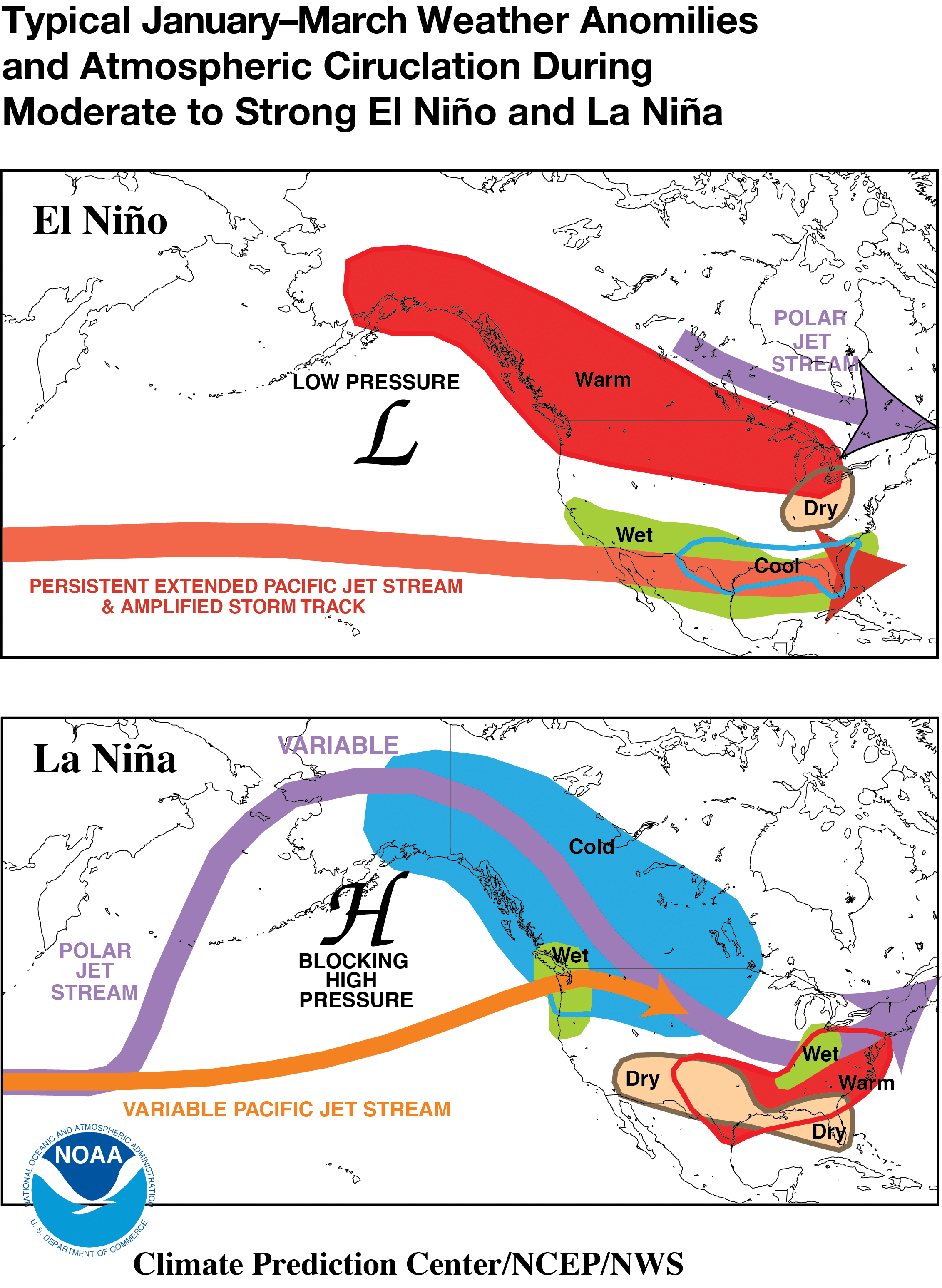 |
| Figure 2-5. Typical January-March weather anomalies and atmospheric circulation during El Niño (top) and La Niña (bottom) events. Image courtesy National Weather Service (NWSa undated). |
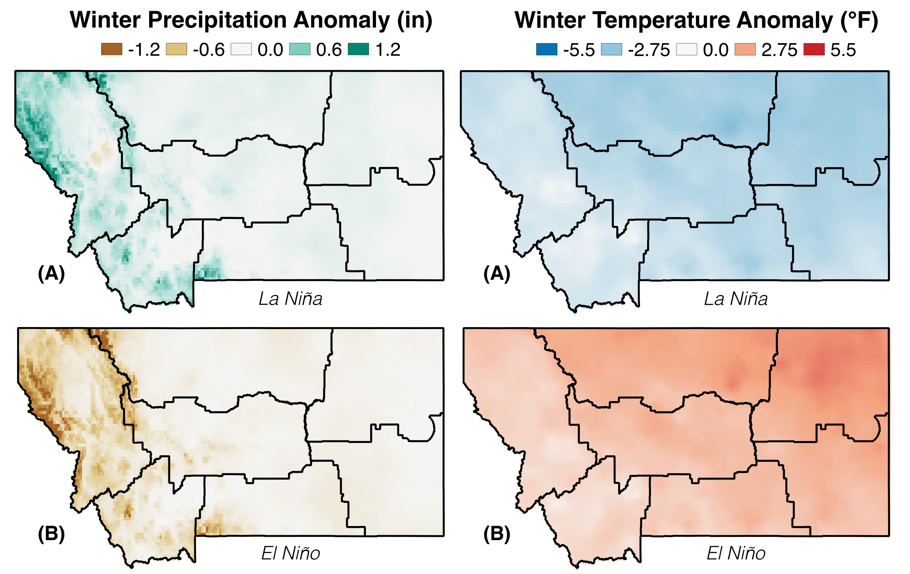 |
| Figure 2-6. (A) Top two images show the average anomaly in Montana’s winter precipitation (left) and temperature (right) during La Niña events. (B) Bottom two images show the average anomaly in Montana’s winter precipitation (left) and temperature (right) during El Niño events. For Montana, El Niño winters are generally drier and warmer; La Niña winters are generally wetter and colder. This analysis was done using data from Livneh et al. (2013) and is based on the study period of 1915-2013. |
Pacific Decadal Oscillation.—The Pacific Decadal Oscillation is a pattern of ocean-atmospheric climate variability across the mid-latitude Pacific Ocean. The oscillation varies in time from interannual to inter-decadal, with the strongest cycle typically occurring about every 30 yr. Effects of the Pacific Decadal Oscillation are not as intense as the El Niño-Southern Oscillation cycle (Mantua and Hare 2002). During its warm phase, winter temperatures are warmer throughout Alaska, western Canada, and the western US (by an average of 2°F [1.1°C]), and precipitation is decreased (Figure 2-7). Effects during the cool phase reverse, with cooler winter temperatures and increased precipitation experienced over western North America.
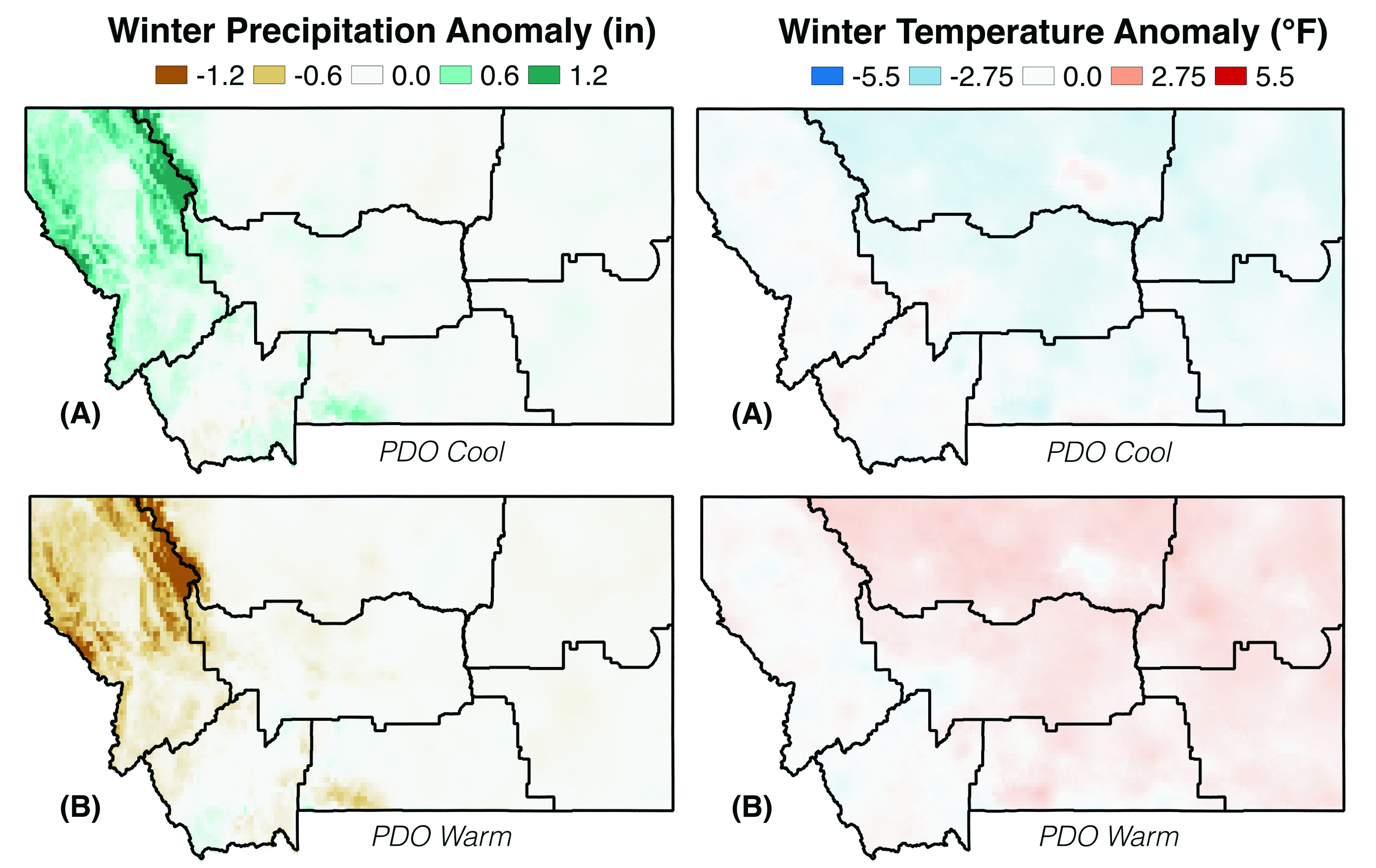 |
| Figure 2-7. (A) Top two images show the average anomaly in Montana’s winter precipitation (left) and temperature (right) during the cool phase of the Pacific Decadal Oscillation. (B) Bottom two images show the average anomaly in Montana’s winter precipitation (left) and temperature (right) during the warm phase of the Pacific Decadal Oscillation. For Montana, the warm phase of the Pacific Decadal Oscillation is generally associated with warmer and drier winters. Cool phase Pacific Decadal Oscillation winters are generally wetter and colder. This analysis was done using data from Livneh et al. (2013) and is based on the study period of 1915-2013. |
The Pacific Decadal Oscillation and El Niño-Southern Oscillation teleconnections may reinforce or moderate each other, depending on if their phases are in alignment or opposition.
Global Climate Modeling
Projecting future climate on a global scale requires modeling many intricate relationships between the land, ocean, and atmosphere. Many global climate and Earth system models exist, each varying in complexity, capabilities, and limitations.
Consider one of the simplest forms of a model used for future projections, a linear regression model (Figure 2-8). With this model, researchers would plot a climate variable (e.g., temperature) over time, draw a best-fit, straight line through the data, and then extend the line into the future. That line, then, provides a means of projecting future conditions. Whether or not those projections are valid is a separate question. For example, the model may be based on false assumptions: the relationship may a) not be constant through time, b) not include outside influences such as human interventions (e.g., policy regulations), and c) not consider system feedbacks that might enhance or dampen the relationship being modeled.
While the linear regression model provides an instructive visual aid for considering modeling, it is too simple for looking at climate changes, in which the interactions are complex and often nonlinear. For example, if temperatures rises, evaporation is expected to increase. At the same time, increasing temperatures increase the atmosphere’s capacity to hold water. Water is a greenhouse gas so more water in the atmosphere means the atmosphere can absorb more heat…thus driving more evaporation. What seemed a simple relationship has changed (possibly dramatically) because of this feedback between temperature, evaporation, and the water-holding capacity of the atmosphere.
Linear models do not account for such nonlinear relationships. Instead, climate scientists account for nonlinearity through computer simulations that describe the physical and chemical interactions between the land, oceans, and atmosphere. These simulations, which project climate change into the future, are called general circulation models (GCMs; see sidebar)
|
General Circulation Models General circulation models (GCMs) help us project future climate conditions. They are the most advanced tools currently available for simulating the response of the global climate system—including processes in the atmosphere, ocean, cryosphere, and land surface—to increasing greenhouse gas concentrations. GCMs depict the climate using a 3-D grid over the globe, typically having a horizontal resolution of between 250 and 600 km (160 and 370 miles), 10-20 vertical layers in the atmosphere and sometimes as many as 30 layers in the oceans. Their resolution is quite coarse. Thus, impacts at the scale of a region, for example for Montana, require downscaling the results from the global model to a finer spatial grid (discussed later) (text adapted from IPCC 2013b). |
||
Because of the complexities involved, climate scientists rarely rely on a single model, but instead use an ensemble (or suite) of models. Each model in an ensemble represents a single description of future climate based on specific initial conditions and assumptions. The use of multiple models helps scientists explore the variability of future projections (i.e., how certain are we about the projection) and incorporate the strengths, as well as uncertainties, of multiple approaches.
For the work of the Montana Climate Assessment, we employed an ensemble from the fifth iteration of the Coupled Model Intercomparison Project (CMIP5), which includes up to 42 GCMs depending on the experiment conducted (CMIP5 undated). The World Climate Research Program describes CMIP as “a standard experimental protocol for studying the output” of GCMs (CMIP undated). It provides a means of validating, comparing, documenting, and accessing diverse climate model results. The CMIP project dates back to 1995, with the fifth iteration (CMIP5) starting in 2008 and providing climate data for the latest IPCC Fifth Assessment Report (Stocker et al. 2013).
We employed 20 individual GCMs from the CMIP5 project for the Montana Climate Assessment ensemble, chosen because they provide daily outputs and a range of important climate variables.9 For this first Montana Climate Assessment, we are only using climate variables of temperature and precipitation (later assessment may evaluate other important variables such as wind and relative humidity).
The benefits of using CMIP5 data are that each model in the ensemble a) has been rigorously evaluated, and b) uses the same standard socioeconomic trajectories—known as Representative Concentration Pathways (RCPs)—to describe future greenhouse gas emissions. RCPs are future greenhouse gas concentration scenarios.
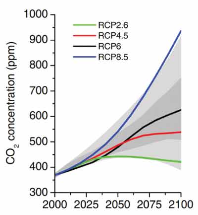
Four RCP scenarios are available in CMIP5: RCP2.6, RCP4.5, RCP6.0, and RCP8.5. The number after RCP represents the increase in radiative forcing in watts/m2 by the year 2100. Higher radiative forcing values are associated with larger amounts of trapped heat in the atmosphere due to increased greenhouse gas emissions (see sidebar). Simply stated, higher RCP values are typically associated with greater greenhouse gas emissions and therefore greater potential for climate change. Each RCP scenario makes different assumptions about future energy sources, population growth, economic activities, and technological advancements, as follows:
- RCP2.6.—The peak-and-decline scenario assumes greenhouse gas emissions peak between 2010-2020 and then decline by the end-of-century, leading to a radiative forcing of 2.6 watts/m2. It assumes greenhouse gas emissions are substantially reduced over time (Van Vuuren et al. 2011).
- RCP4.5.—The stabilization scenario where technological advancements and strategies lead to a peak in greenhouse gas emissions at about 2040 followed by a decline (Clarke et al. 2007). We explore the RCP4.5 scenario in this assessment, and the United Nations Paris Agreement of 2016 curbs emissions at a level between RCP2.6 and RCP4.5.
- RCP6.0.—A second stabilization scenario, but in this pathway greenhouse gas emissions peak at 2080 and stabilization is not achieved until after 2100 (Fujino et al. 2006).
- RCP8.5.—The business-as-usual emission scenario where greenhouse gas emissions increase throughout the 21st century (Riahi et al. 2007, 2009), based on the assumption that society is largely unsuccessful in curbing those emissions. We use the RCP8.5 scenario, in which greenhouse gases steadily rise, and note that this pathway best matches current trends.
|
Representative Concentration Pathways Representative Concentration Pathways (RCPs) make different assumptions about energy sources, population growth, economic activities, and technological advancements. Scientists run general circulations models against these scenarios to project future climate conditions, including atmospheric carbon concentrations. For this Montana Climate Assessment, we considered the stabilization (RCP4.5) and business-as-usual (RCP8.5) emission pathways.
This graph illustrates the different atmospheric CO2 concentrations associated with each Representative Concentration Pathways. For example, if we continue our carbon emissions at the current rate (i.e., the business-as-usual [RCP8.5] emission scenario), the atmospheric CO2 concentration will be roughly 700 ppm by 2075 (IPCC 2014). |
||
For the Montana Climate Assessment, we explore the RCP4.5 and RCP8.5 scenarios only. We do not include RCP6.0 or RCP2.6 in our assessment for several reasons. RCP6.0 overlaps with RCP4.5 in the first half of the century and provides intermediate values between RCP4.5 and RCP8.5 at the end of the century. Additionally, RCP2.6 is becoming less and less realistic as society continues with business as usual regarding greenhouse gas emissions. For the remainder of the chapter, we will regularly refer to RCP4.5 and RCP8.5 as the stabilization and business-as-usual emission scenarios, respectively.
Due to their complexity and global extent, GCMs can be computationally intensive. Thus, scientists often make climate projections at coarse spatial resolution where each projected data point is an average value of a grid cell that measures hundreds of miles (kilometers) across.
For areas where the terrain and land cover are relatively homogenous (e.g., an expanse of the Great Plains), such coarse grid cells may be adequate to capture important climate processes. But in areas with complex landscapes like Montana, data points so widely spaced are inadequate to reflect variability in terrain and vegetation and their influence on climate. A 100 mile (161 km) grid, for example, might not capture the climate effects of a small mountain range rising out of the eastern Montana plains or the climate differences between mountain summits and valleys in western Montana where temperature and precipitation vary greatly.
To capture such important terrain characteristics, scientist take the coarse-resolution output from a GCM and statistically attribute the results from those models to smaller regions at higher resolution (e.g., grid points at 1 mile rather than 100 mile apart). This process, called downscaling, more accurately represents climate across smaller, more complex landscapes, including Montana.
For this climate assessment, we used a statistical downscaling method called the Multivariate Adaptive Constructive Analogs.10 By using a downscaled dataset—rather than the original output from the ensemble of GCMs—we gained the ability to evaluate temperature and precipitation at relatively high resolution statewide before conveying the results at the climate division scale. Additionally, we were able to aggregate data points within each of Montana’s seven climate divisions (Figure 2-3), and look at Montana’s climate future in different geographic areas. Aggregating to the climate-division level minimizes the potential for false precision by reporting results at spatial scales that better represent underlying climate processes.
The 20-downscaled GCMs in CMIP5 were evaluated at two future time periods: 1) mid century (2040–2069) and 2) end-of-century (2070–2099). Thirty-year averages of these future projections were then compared to a historical (1971–2000) 30-year average, which results in a projected difference, or change, from historical conditions. We make those projections using the stabilization (RCP4.5) and business-as-usual (RCP8.5) emission scenarios described previously (see sidebar). These future projections were then compared to the historical trends in Montana to reveal the major climate-associated changes that Montana is likely to experience in the future.
|
|
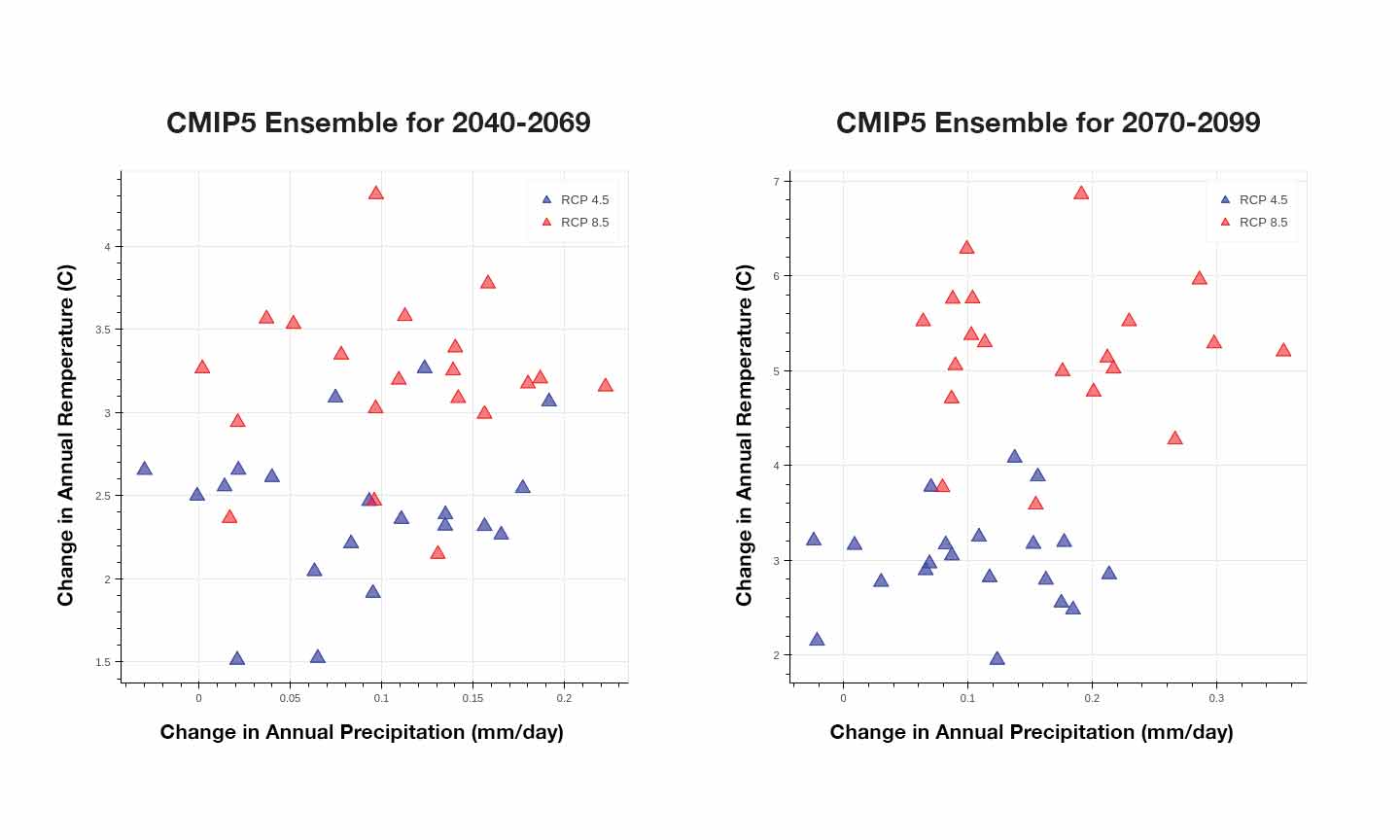
Modeling Montana’s Climate Future To derive the climate projections for this assessment, we employed 20 general circulation models to consider two scenarios of global carbon emissions: one where atmospheric greenhouse gases are stabilized by the end of the century and the other where it grows on its current path (the stabilization [RCP4.5] and business-as-usual [RCP8.5] emission scenarios, respectively).
Model output summary from the 20 GCMs that compares projected changes in temperature and precipitation for the state of Montana for stabilization (RCP4.5 – blue symbols) and business-as-usual (RCP8.5 – red symbols) emission scenarios between (A) mid century (2040-2069), and (B) end-of-century (2070-2099).
As shown in the figures above, we forecast Montana’s future climate for two periods: mid century and end-of-century. In brief:
|
|
Temperature projections
Below we provide projections for various aspects of Montana’s future temperature based on our modeling analysis. These projections are for the stabilization (RCP4.5) and business-as-usual (RCP8.5) emission scenarios and for two periods: mid century (2040-2069) and end-of-century (2070-2099).
We discuss a subset of our modeling results here, including a) temperature projections reported by the median values of the 20 GCM ensemble and b) figures that include maps and graphs that represent the median value and distribution of values observed for temperature across the 20 GCMs.
An ensemble minimum, maximum, and percent agreement are also provided parenthetically. The percent agreement represents the number of GCMs that project the same sign of change (i.e., positive or negative) as the median value. For example, if the median value is positive and 18 out of 20 models also project positive change, then the percent agreement would be 100 x 18/20 = 90%. This simple calculation helps convey the uncertainty in the projections.
Average annual temperatures
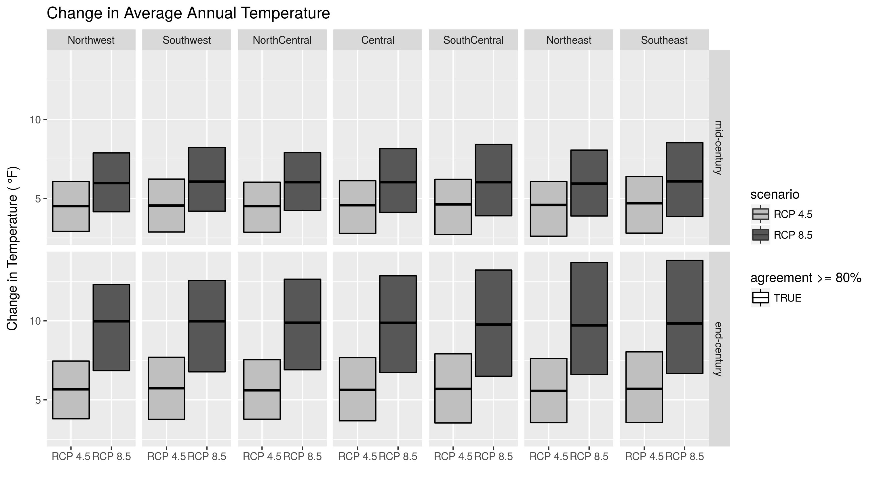
Average annual temperatures increase in the mid-century and end-of-century projections for both stabilization and business-as-usual emission scenarios (Figures 2-9, 2-10). In the mid-century projection, most of the state has increases of about 4.5°F (2.5°C) for the stabilization emission scenario and 6.0°F (3.3°C) for the business-as-usual emission scenario. For end-of-century, statewide temperature increases by about 5.6°F (3.1°C) for the stabilization emission scenario and 9.8°F (5.4 °C) for the business-as-usual emission scenario. Although small differences exist between climate divisions, the general magnitude of these changes is consistent across the state for both emission scenarios and both time periods.
- Mid-century projection specifics.—Average annual temperatures increase by mid century in both emission scenarios (Figures 2-9 and 2-10). In the stabilization emission scenario, most of the state is projected to have increases of about 4.5°F (2.5°C) (minimum: 2.7°F [1.5°C], maximum: 6.1°F [3.4°C], percent agreement: 100%). The business-as-usual emission scenario projects larger increases in temperature of about 6.0°F (3.3°C) (minimum: 4.0°F [2.2°C], maximum: 8.2°F [4.6°C], model agreement: 100%). While small discrepancies exist between climate divisions, in general the magnitude of these changes is consistent across the state in both emission scenarios.
- End-of-century projection specifics.—Average annual temperatures increase by about 5.6°F (3.1°C) (minimum: 3.6°F [2.0°C], maximum: 7.7°F [4.3°C], percent agreement: 100%) in the stabilization emission scenario and by about 9.8°F (5.4°C) (minimum: 6.6°F [3.7°C], maximum: 12.9°F [7.2°C], percent agreement: 100%) in the business-as-usual emission scenario (Figure 2-9).
|
|
| Figure 2-9. Graphs showing the minimum, maximum, and median temperature increases (°F) projected for each climate division in both stabilization (RCP4.5) and business-as-usual (RCP8.5) emission scenarios. The top row shows mid-century (2040-2069) projections and the bottom row shows end-of-century (2070-2099) projections. The outline of each box is determined by model agreement on the sign of the change (positive or negative). A black outline means there is >=80% model agreement and a red outline means that there is <80% model agreement. In this case, all models indicated the direction of the temperature trend at an agreement of greater than 80%. |
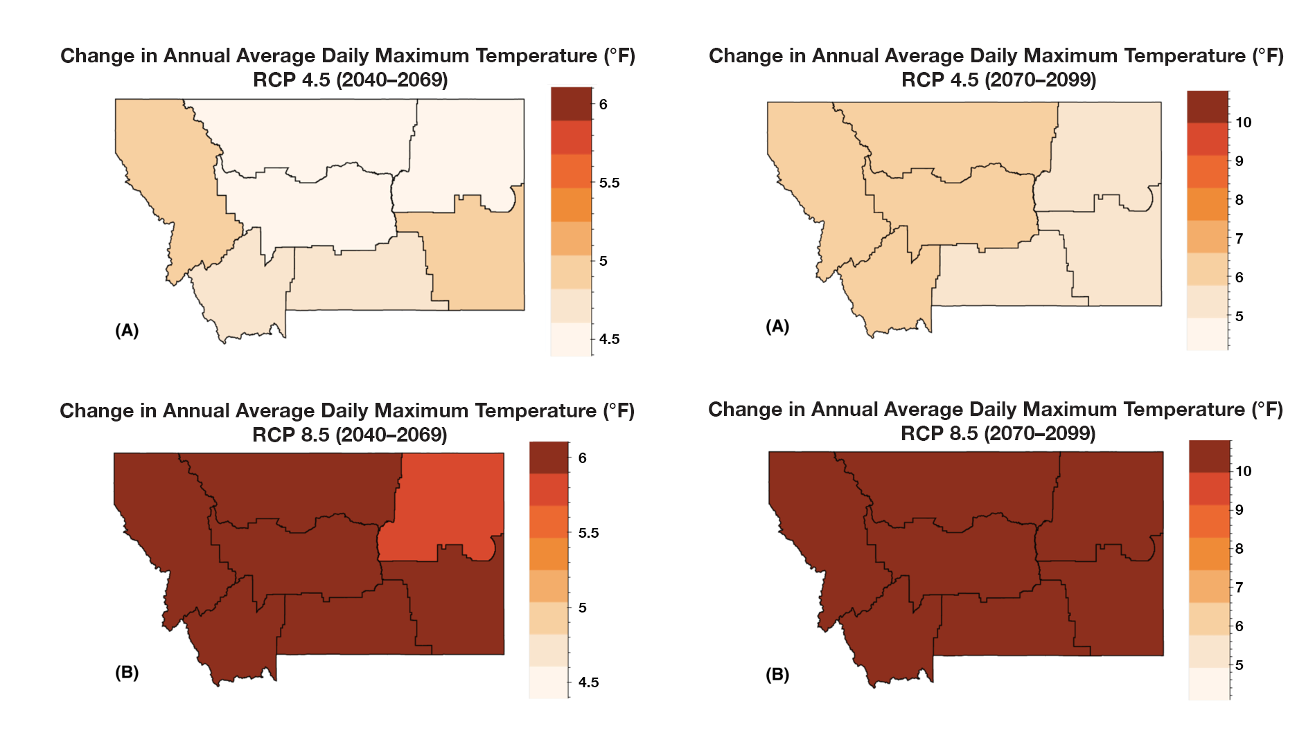
Average daily minimum and maximum temperatures
Average daily minimum and maximum temperatures increase in the mid-century and end-of-century projections for both stabilization and business-as-usual emission scenarios (Figure 2-10 shows output for annual average daily maximum temperature). The degree of change is similar to that found for the average annual temperatures. In end-of-century projections, summers have the largest increases in average temperature: 6.5°F (3.6°C) for the stabilization emission scenario, 11.8°F (6.6°C) for the business-as-usual emission scenario.
- Mid-century projection specifics.—Average daily minimum and maximum temperatures change in a manner similar to the average annual projected increases (again for both RCP scenarios).
- End-of-century projection specifics.—Average daily minimum and maximum temperatures increase by similar magnitudes to average annual daily temperatures for both emission scenarios. Summer months have the largest projected increase in average temperature. In the stabilization emission scenario, summer temperatures increase by 6.5°F (3.6°C) (minimum: 3.2°F [1.8°C], maximum: 9.1°F [5.1°C], percent agreement: 100%) and in the business-as-usual emission scenario, summer temperatures increase by about 11.8°F (6.6°C) (minimum: 8.0°F [4.4°C], maximum: 15.2°F [8.4°C], percent agreement: 100%).
|
Mid-century and End-of-century |
| Figure 2-10. The projected increase in annual average daily maximum temperature (°F) for each climate division in Montana for the periods 2049-2069 and 2070-2099 for (A) stabilization (RCP4.5) and (B) business-as-usual (RCP8.5) emission scenarios. |
Average monthly temperatures
Average monthly temperatures are projected to increase across all climate divisions by mid century (2040-2069) and for both stabilization and business-as-usual emission scenarios (Figure 2-11). Average monthly temperatures in summer and winter generally show larger projected increases than those in spring and fall. In the business-as-usual emission scenario, August has the largest projected change across all climate divisions.
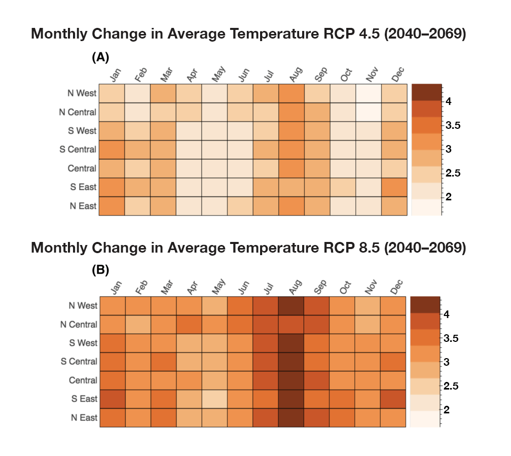 |
| Figure 2-11. The projected monthly increase in average temperature (°F) for each climate division in Montana in the mid-century projections (2040-2069) for the (A) stabilization (RCP4.5) and (B) business-as-usual (RCP8.5) emission scenarios. |
The number of days above 90°F (32°C)
The number of annual days where maximum temperatures are above 90°F (32°C) increases across all climate divisions in both mid-century and end-of-century projections and for both stabilization and business-as-usual emission scenarios (Figures 2-12, 2-13). Large differences in the magnitude of change exist, however, among the climate divisions. For example, in mid-century projections using the business-as-usual emission scenario, the northwestern part of the state shows increases of about 11 days with temperatures above 90°F (32°C), while the eastern parts of the state have increases of about 33 days. Similarly, in end-of-century projections based on the business-as-usual emission scenario, the northwestern part of the state shows an increase of about 34 days, while the eastern parts of the state have an increase of about 54 days above 90°F (32°C).
- Mid-century projection specifics.—The number of annual days at mid century where maximum temperatures are above 90°F (32°C) increases across all climate divisions and both emission scenarios (Figure 2-12, 2-13). Large differences in the magnitude of change exist, however, among the climate divisions. These differences are likely due, in part, to variability in moisture availability among the climate divisions and the energy it takes to evaporate this moisture (i.e., latent heat). In the stabilization emission scenario, the northwestern and north central climate divisions have increases of about 5.0 days (minimum: 1.5 days, maximum: 12.0 days, percent agreement: 100%); while the number of days in both eastern and south central climate divisions of the state increase by about 25.0 days (minimum: 6.0 days, maximum: 36.0 days, percent agreement: 100%). Similar spatial patterns exist for the business-as-usual emission scenario, but the magnitudes of change increase along with the ranges of the ensemble minimums and maximums. In the northwestern and north central climate divisions of the state, increases of about 11 days are projected (minimum: 1.5 days, maximum: 25.0 days, percent agreement: 100%); in the south central and both eastern climate divisions increases are projected to be about 33.0 days (minimum: 11 days, maximum: 44.0 days, percent agreement: 100%).
- End-of-century projection specifics.—The number of days where maximum temperatures exceed 90°F (32°C) by the end-of-century continues to increase across the state in both emission scenarios, with 100% model agreement. The spatial pattern in the end-of-century projection is similar to that of the mid-century one (Figures 2-12, 2-13). For the stabilization emission scenario, the number of days/yr exceeding 90°F (32°C) increases in the northwestern and north central regions by about 8.5 days (minimum: 1.7 days, maximum: 22.0 days, percent agreement: 100%), while in the southern and eastern parts of the state, it increases by about 29.0 days (minimum: 11.0 days, maximum: 43.0 days, percent agreement: 100%). For the business-as-usual emission scenario, the number of days exceeding 90°F (32°C) in the northwestern and north central parts of the state increases by about 34.0 days (minimum: 9.5 days, maximum: 58.0 days, percent agreement: 100%), while in the southern and eastern parts of the state, it increases by about 54.0 days (minimum: 26.0 days, maximum: 70.0 days, percent agreement: 100%).
Mid-century and End-of-century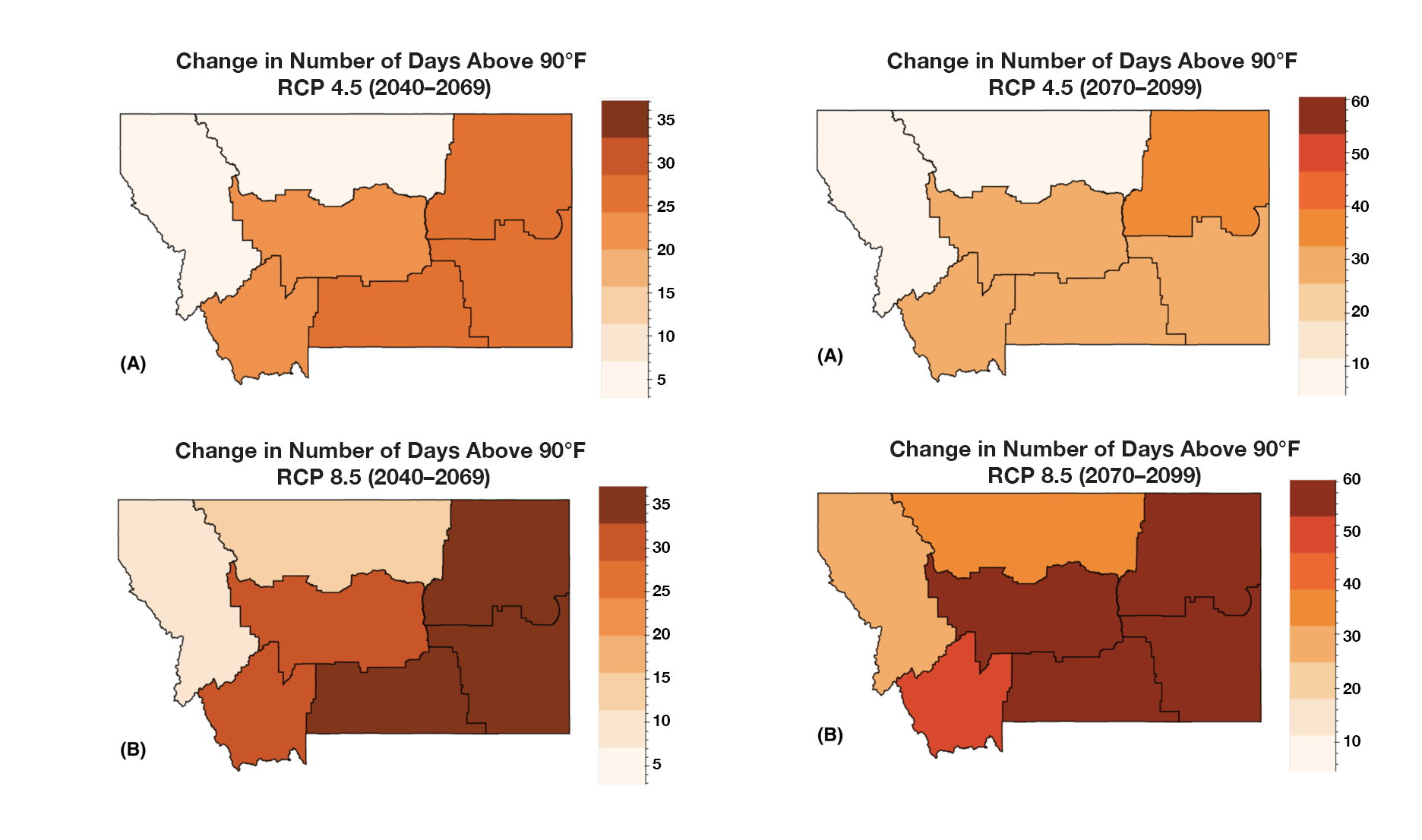 |
| Figure 2-12. The projected increases in number of days above 90°F (32°C) for each climate division in Montana over two periods 2040-2069 and 2070-2099 for (A) stabilization (RCP4.5) and (B) business-as-usual (RCP8.5) emission scenarios. |
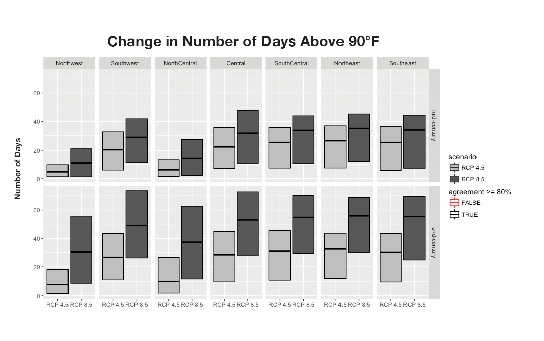 |
| Figure 2-13. Graphs showing the increase in the number of days per year above 90°F (32°C) projected for each climate division in both stabilization (RCP4.5) and business-as-usual (RCP8.5) emission scenarios. The top row shows mid-century projections (2040-2069) and the bottom row shows end-of-century projections (2070-2099). The outline of each box is determined by model agreement on the sign of the change (positive or negative). A black outline means there is ≥80% model agreement and a red outline means that there is <80% model agreement. In this case, all models indicated the direction of the trend for days above 90°F (32°C) at an agreement of greater than 80%. |
Number of days where minimum temperatures are above 32°F (0°C)
The number of days/yr where minimum temperatures exceed 32°F (0°C; i.e., frost-free days) also increases across all climate divisions in both mid- and end-of-century projections and for both stabilization and business-as-usual emission scenarios (Figures 2-14, 2-15). While varying considerably across the state, projected changes are substantial. For example, in the mid-century projections with the stabilization emission scenario, frost-free days increase by about 30 days in the western part of the state and by 23 days in the eastern part of the state. Similar patterns exist for end-of-century projections: in the business-as-usual emission scenario, frost-free days increase by about 70 days in the western part of the state and by about 55 days in the eastern part of the state.
- Mid-century projection specifics.—The number of days/yr where minimum temperatures are above 32°F (0°C; i.e., frost-free days) increases across all climate divisions and both emission scenarios (Figures 2-14, 2-15). In the stabilization emission scenario, frost-free days increase by 30.0 days in the western part of the state (minimum: 9.0 days, maximum: 51.0 days, percent agreement: 100%) and by 23.0 days in the eastern part of the state (minimum: 10.0 days, maximum: 43.0 days, percent agreement: 100%). In the business-as-usual emission scenario, frost-free days increase by 41.0 days in the western part of the state (minimum: 17.0 days, maximum: 68.0 days, percent agreement: 100%) and by 32.0 days in the eastern part of the state (minimum: 15.0 days, maximum: 63.0 days, percent agreement: 100%).
- End-of-century projection specifics.—The number of days/yr where minimum temperatures are above 32°F (0°C; i.e., frost-free days) continues to increase in the end-of-century projections across all climate divisions and for both emission scenarios, with 100% model agreement. Again, similar spatial patterns exist between the mid-century and end-of-century projections (Figures 2-14, 2-15). In the stabilization emission scenario, frost-free days increase by 41.0 days in the western part of the state (minimum: 18.0 days, maximum: 66.0 days, percent agreement: 100%), and by 30.0 days in the eastern part of the state (minimum: 14.0 days, maximum: 60.0 days, percent agreement: 100%). In the business-as-usual emission scenario, frost-free days increase by 70.0 days in the western part of the state (minimum: 36.0 days, maximum: 110.0 days, percent agreement: 100%), and by 55.0 days in the eastern part of the state (minimum: 26.0 days, maximum: 100.0 days, percent agreement: 100%).
Mid-century and End-of-century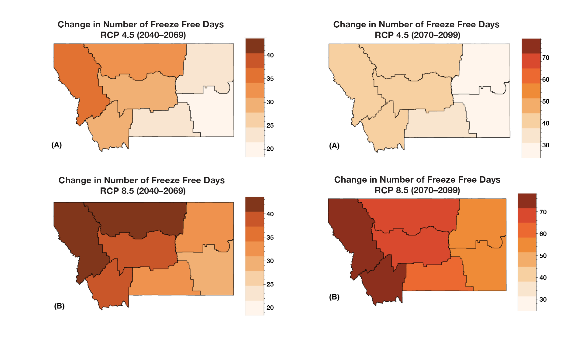 |
| Figure 2-14. The projected change in the number of frost-free days for each climate division in Montana over two periods 2040-2069 and 2070-2099 for (A) stabilization (RCP4.5) and (B) business-as-usual (RCP8.5) emission scenarios. |
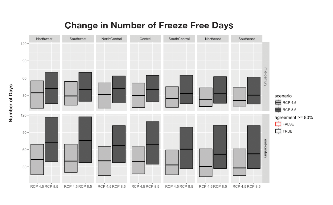 |
| Figure 2-15. Graphs showing the increases in frost-free days/yr projected for each climate division in both stabilization (RCP4.5) and business-as-usual (RCP8.5) emission scenarios. The top row shows mid-century projections (2040-2069) and the bottom row shows end-of-century projections (2070-2099). The outline of each box is determined by model agreement on the sign of the change (positive or negative). A black outline means there is >=80% model agreement and a red outline means that there is <80% model agreement. In this case, all models indicated the direction of the trend of frost-free days at an agreement of greater than 80%. |
Summary
In general, there is high model agreement and low uncertainty that temperatures and associated temperature metrics will increase both by mid century and end-of-century. For both periods, annual and seasonal temperature averages, the number of days/yr with extreme heat, and the overall length of the growing season are projected to increase. Differences exist in projections for the stabilization and business-as-usual emission scenarios, with the former consistently showing lower magnitudes of change than the latter. Many of the trends and spatial patterns seen in the mid-century projections are extended and exacerbated in the end-of-century projections. The range of model outputs also increases for end-of-century projections, suggesting that the magnitude of change becomes more uncertain in the models further out in time.
Regardless of uncertainties, the GCMs show full agreement regarding the direction of change: temperatures will be increasing.
Precipitation projections
Below we provide projections of Montana’s future precipitation based on our modeling efforts. Those projections are for the stabilization and business-as-usual emission scenarios and for two periods: mid century (2040-2069) and end-of-century (2070-2099).
We discuss a subset of our precipitation modeling results here, including a) precipitation projections reported by the median values of the 20 GCM ensemble and b) figures that include maps and graphs that represent the median value and distribution of values observed for precipitation across the 20 GCMs. Special consideration is required for interpretations of precipitation changes in Montana’s complex terrain. Precipitation increases drastically with elevation such as that found in northwest Montana. Here, median values do not characterize the potential for spatial variability that exists within these regions.
An ensemble minimum, maximum, and percent agreement are also provided parenthetically. As with our temperature analysis, the percent agreement concerning the precipitation trends is based on the number of GCMs that project the same sign of change (i.e., positive or negative) as the median value. For example, if the median value is positive and 18 out of 20 models also project positive change, then the percent agreement would be 100 x 18/20 = 90%. This simple calculation helps convey the uncertainty in the projections. For some variables both the absolute change and the percent change from historical is calculated.
Average annual precipitation
Average annual precipitation increases across the state in both mid-century and end-of-century projections for both emission scenarios (Figures 2-16, 2-17, 2-18). For the mid-century projection using the stabilization emission scenario, increases of about 1.3 inch/yr (3.3 cm/yr) occur in the northwestern and north central climate divisions and about 0.9 inch/yr (2.3 cm/yr) in the southwestern, central, and eastern climate divisions. For the business-as-usual emission scenario in the mid-century projection, average annual precipitation increases by about 2.0 inch/yr (5.1 cm/yr) in the western half of the state, and about 1.8 inch/yr (4.6 cm/yr) in the eastern half of the state. The GCMs used in the ensemble show large differences in their end-of-century projections, but there is high agreement in the positive direction of change.
- Mid-century projection specifics.—Average annual precipitation increases by mid century across the state for both emission scenarios, with moderately high agreement among models (Figures 2-16, 2-17, 2-18). In the stabilization scenario, increases of about 1.3 inch/yr (3.3 cm/yr) and 5.0% (minimum: -0.5 inch/yr [-1.3 cm/yr], -1.1%; maximum: 3.2 inch/yr [8.1 cm/yr], 14.0%; percent agreement: 85%) are projected in the northwestern parts of the state. In the southern and eastern parts of the state, increases of about 0.9 inch/yr (2.3 cm/yr) and 6.5% are projected (minimum: -1.2 inch/yr [-3.0 cm/yr], -6.0%; maximum: 2.5 inch/yr [6.4 cm/yr], 18.0%; percent agreement: 85%). In the business-as-usual emission scenario, average annual precipitation increase by about 1.6 inch/yr (4.1 cm/yr) and 6.5% in the northwestern parts of the state (minimum: -0.2 inch/yr [-0.51 cm/yr], -1.0%; maximum: 4.4 inch/yr [11.2 cm/yr], 17.0%; percent agreement: 90%), and by about 1.2 inch/yr (3.0 cm/yr) and 10% in the southern and eastern parts of the state (minimum: -0.5 inch/yr [-1.3 cm/yr], -3.5%; maximum: 2.9 inch/yr [7.4 cm/yr], 22.0%; percent agreement: 85%).
- End-of-century projection specifics.—Average annual precipitation is projected to increase through the end-of-century for both emission scenarios (Figures 2-16, 2-17, 2-18). The GCMs used in the ensemble show large differences in their end-of-century projections, but there is high agreement in the positive direction of change. In the stabilization emission scenario, average annual precipitation increases in the northwestern climate division by about 2.2 inch/yr (5.6 cm/yr) and 7.3% (minimum: -1.2 inch/yr [-3.0 cm/yr], -4.5%; maximum: 3.6 inch/yr [9.1 cm/yr], 12.9%; percent agreement: 85%), and by about 1.1 inch/yr (2.8 cm/yr) and 8.0% in the two eastern climate divisions (minimum: -0.5 inch/yr [-1.3 cm/yr], -4.5%; maximum: 3.0 inch/yr [7.6 cm/yr], 18.0%; percent agreement: 85%). In the business-as-usual emission scenario, average annual precipitation is projected to increase by slightly more than in the stabilization emission scenario, although the range of model projections also increases. In the western half of the state, annual precipitation increases by about 2.0 inch/yr (5.1 cm/yr) and 10.0% (minimum: 0.4 inch/yr [1.0 cm/yr], 1.3%; maximum: 5.5 inch/yr [14.0 cm/yr], 28.0%; percent agreement: 100%), and in the eastern half of the state annual precipitation increases by about 1.8 inch/yr (4.6 cm/yr) and 14.0% (minimum: -0.2 inch/yr [-0.5 cm/yr], -1.0%; maximum: 3.6 inch/yr [9.1 cm/yr], 26.0%; percent agreement: 95%).
|
Mid-century and End-of-century |
| Figure 2-16. The projected change in annual precipitation (inches) for each climate division in Montana over two periods 2040-2069 and 2070-2099 for (A) stabilization (RCP4.5) and (B) business-as-usual (RCP8.5) emission scenarios. |
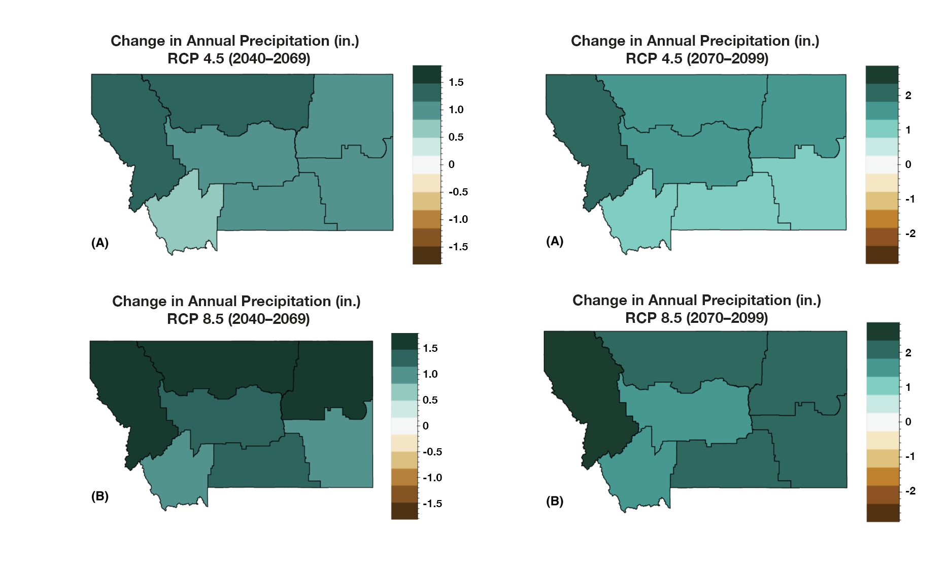
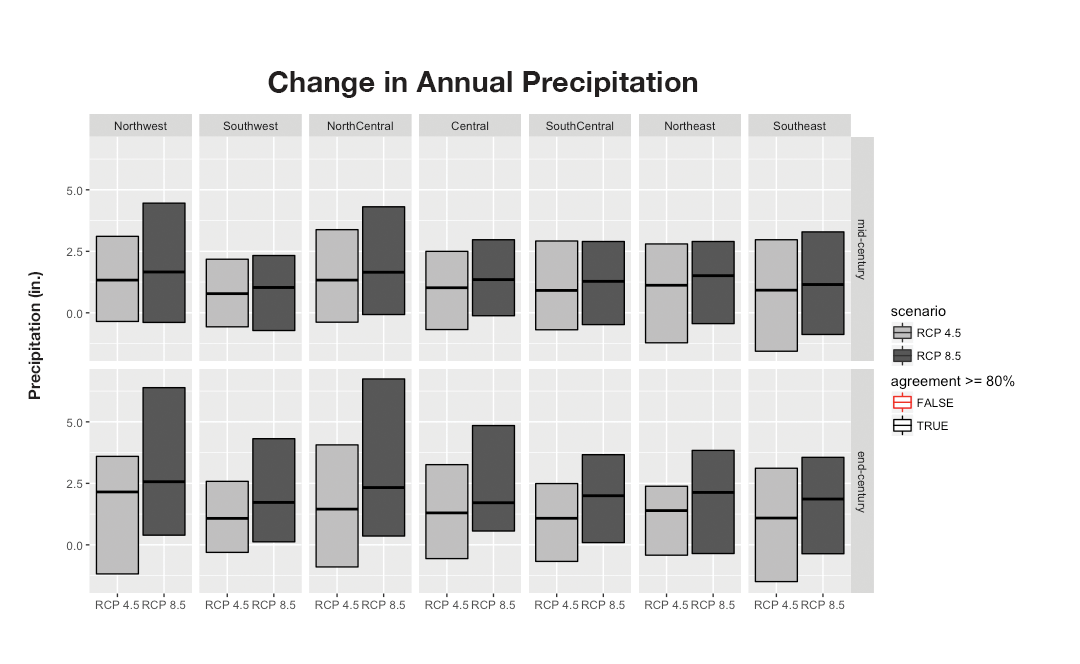 |
| Figure 2-17. Graphs showing annual precipitation change (in inches) projected for each climate division in both stabilization (RCP4.5) and business-as-usual (RCP8.5) emission scenarios. The top row shows mid-century projections (2040-2069) and the bottom row shows end-of-century projections (2070-2099). The outline of each box is determined by model agreement on the sign of the change (positive or negative). A black outline means there is >=80% model agreement and a red outline means that there is <80% model agreement. In this case, all models indicated the direction of the annual precipitation trend at an agreement of greater than 80%. |
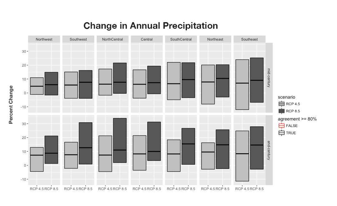 |
| Figure 2-18. Graphs showing the minimum, maximum, and median percent changes in annual precipitation projected for each climate division in both stabilization (RCP4.5) and business-as-usual (RCP8.5) emission scenarios. The top row shows mid-century projections (2040-2069) and the bottom row shows end-of-century projections (2070-2099). The outline of each box is determined by model agreement on the sign of the change (positive or negative). A black outline means there is >=80% model agreement and a red outline means that there is <80% model agreement. In this case, all models indicated the direction of the precipitation trend at an agreement of greater than 80%. |
Interannual variability
Interannual variability (i.e., the amount precipitation changes from year to year) is also projected to increase slightly across the state by mid century and end-of-century for both emission scenarios (Figure 2-19). The increase could be attributed to wet years getting wetter, dry years getting drier, or some combination of both.
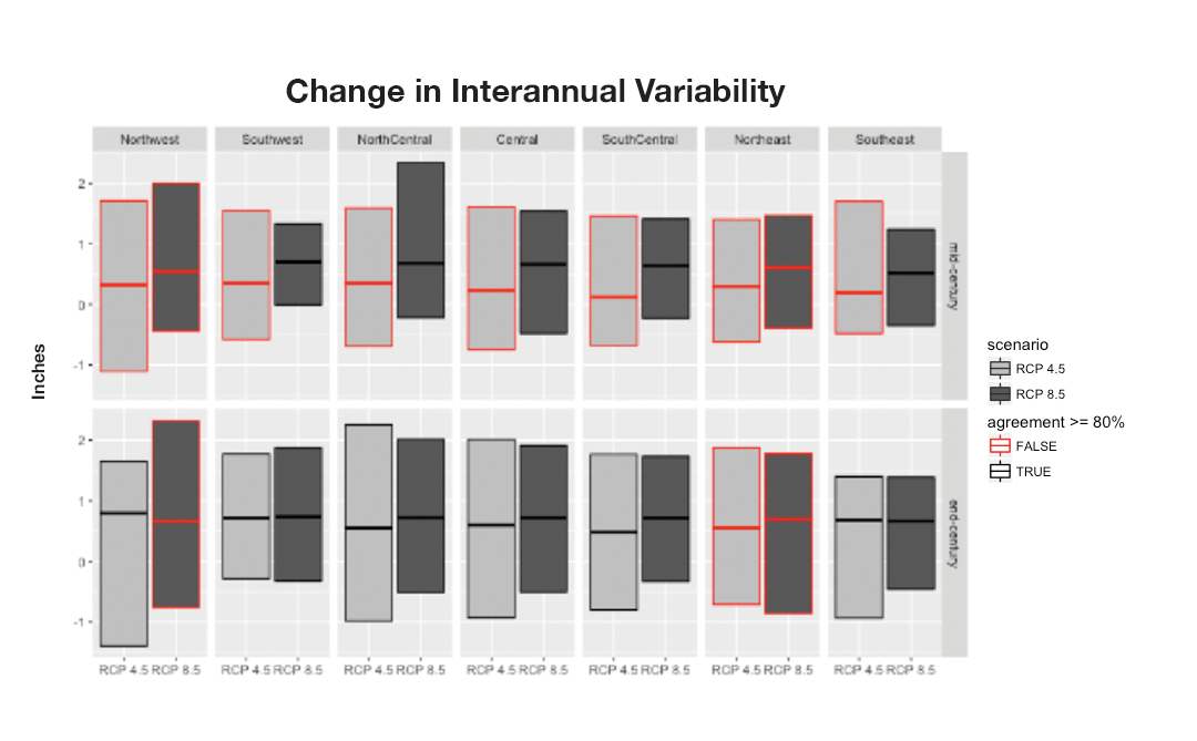 |
| Figure 2-19. Graphs showing the interannual variability of precipitation projected for each climate division in both stabilization (RCP4.5) and business-as-usual (RCP8.5) emission scenarios. The top row shows mid-century projections (2040-2069) and the bottom row shows for end-of-century projections (2070-2099). The outline of each box is determined by model agreement on the sign of the change (positive or negative). A black outline means there is ≥80% model agreement and a red outline means that there is <80% model agreement. |
Monthly and seasonal change in average precipitation
While annual increases in precipitation are projected across the state with moderately high model agreement, the monthly and seasonal projections vary. In mid-century projections, winter, spring, and fall increase in monthly precipitation for both emission scenarios, with spring experiencing the largest increases (e.g., 0.4 inch/month [1.0 cm/month] for the business-as-usual emission scenario; Figure 2-23). Summers, however, are projected to decrease by about 0.1 inch/month (0.3 cm/month) in both emission scenarios (model agreement, however, is fairly low for these projections). For end-of-century projections, the same trends are seen for increasing precipitation in winter, spring, and fall and decreasing precipitation in summer. The magnitude of change is similar to that of mid-century projections.
|
|
| Figure 2-20. Projected monthly change in average precipitation (inches) for each climate division in Montana in the mid-century projections (2040-2069) for (A) stabilization (RCP4.5) and (B) business-as-usual (RCP8.5) emission scenarios. |
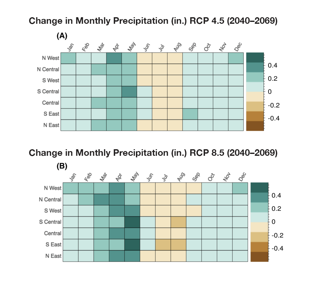
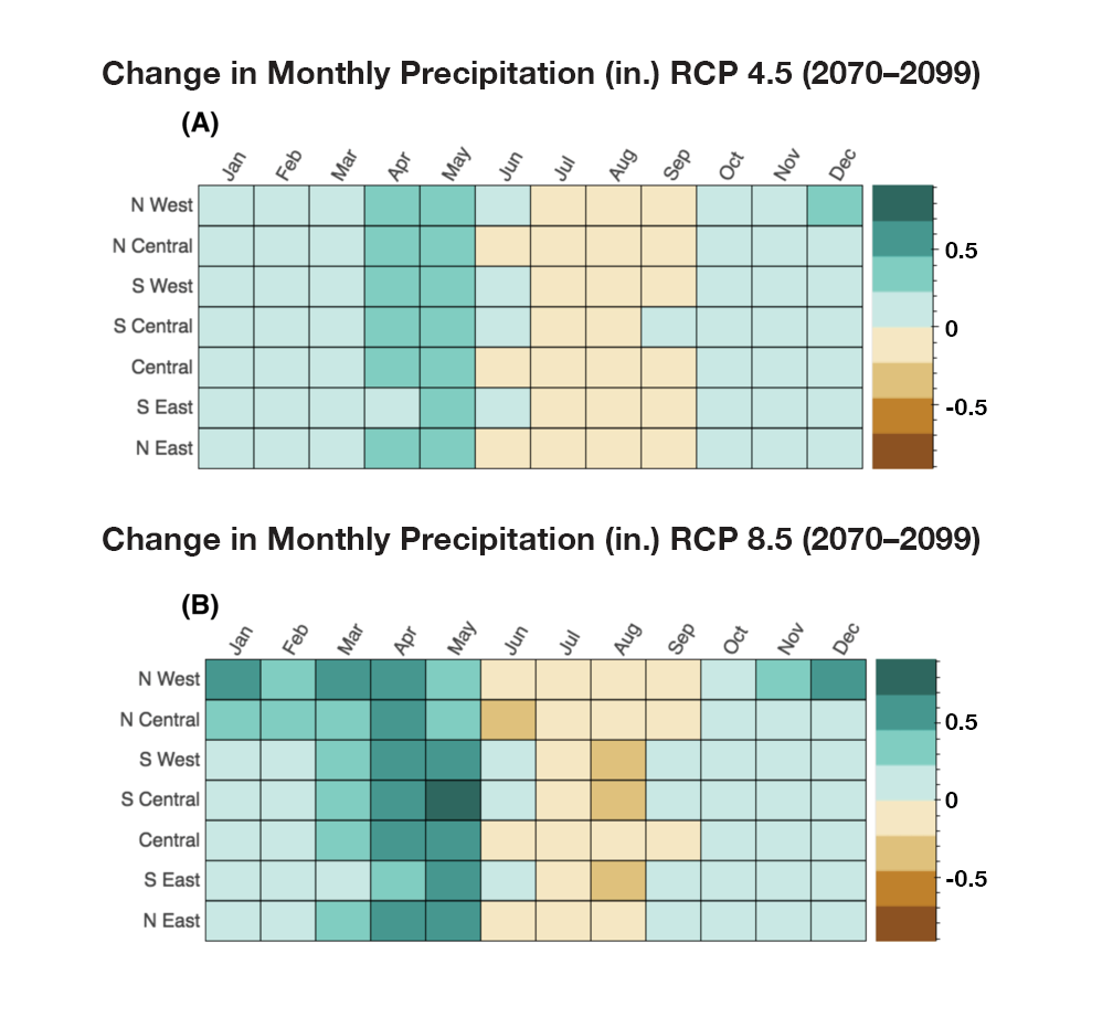 |
| Figure 2-21. The projected monthly change in average precipitation (inches) for each climate division in Montana in the end-of-century projections (2070-2099) for (A) stabilization (RCP4.5) and (B) business-as-usual (RCP8.5) emission scenarios. |
- Mid-century projection specifics.—Although annual precipitation increases across the state with moderately high model agreement, the monthly and seasonal projections vary somewhat. Winter, spring, and fall increase in monthly precipitation for both emission scenarios, with the largest increases in spring (Figure 2-20). For the stabilization emission scenario, spring months increase by about 0.2 inch/month (0.5 cm/month) (minimum: -0.1 inch/month [-0.3 cm/month], maximum: 0.8 inch/month [2.0 cm/month], percent agreement: 85%). In the business-as-usual emission scenario, spring months increase by 0.4 inch/month (1.0 cm/month) (minimum: 0.0 inch/month [0 cm/month], maximum: 1.0 inch/month [2.5 cm/month], percent agreement: 95%). Summer months, however, show decreasing precipitation for both scenarios, although model agreement is fairly low in the projections. For the both the stabilization and business-as-usual emission scenarios, summer precipitation decreases by -0.1 inch/month (-0.3 cm/month) (minimum: -0.4 inch/month [-1.0 cm/month], maximum: 0.5 inch/month [1.3 cm/month], percent agreement: 65%).
- Figure 2-21. The projected monthly change in average precipitation (inches) for each climate division in Montana in the end-of-century projections (2070-2099) for (A) stabilization (RCP4.5) and (B) business-as-usual (RCP8.5) emission scenarios.
Projected change in consecutive dry days
To assess changes in the frequency of dry events, we determined the annual number of dry days (defined as days when precipitation is less than 0.01 inch [0.03 cm]), then calculated the maximum number of consecutive dry days/yr averaged over the 30-year periods of interest. In general, in both mid- and end-of-century projections, we found a modest increase statewide in consecutive dry days—generally less than 0.5 days—for both emission scenarios (Figures 2-22, 2-23). Low model agreement exists and the range of projections from the ensemble of GCMs is wide, both suggesting high uncertainty in these projections.
- Mid-century projection specifics.—In general, consecutive dry days show a modest increase (i.e., less than 0.5 days); however, model agreement is low (approximately 60%; where 50% would mean complete disagreement among models) in both emission scenarios.
- End-of-century projection specifics.—In end-of-century projections, changes in consecutive dry days/yr remain positive, but the increase is small (generally less than 0.5 days) with low model agreement (approximate 60%). This result is consistent across both emission scenarios. The range of projections from the ensemble of models is wide; however, minimum and maximum values are projected to increase by about -2.5 days and 4.0 days, respectively. This large range, in addition to the low model agreement, suggests high uncertainty in these projections.
|
Mid-century and End-of-century |
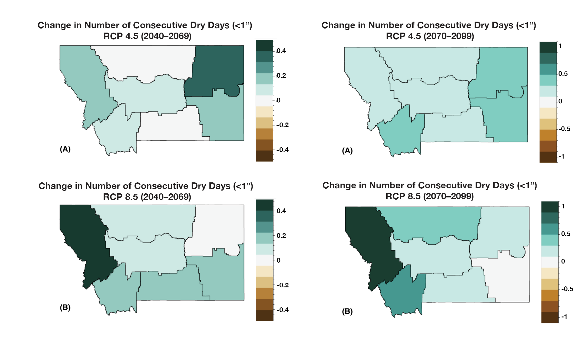 |
| Figure 2-22. The projected change in the number of consecutive dry days (<0.1 inch [0.3 cm] of precipitation) for each climate division in Montana over two periods 2040-2069 and 2070-2099 for (A) stabilization (RCP4.5) and (B) business-as-usual (RCP8.5) emission scenarios. |
|
|
| Figure 2-23. Graphs showing the number of consecutive dry days in a year projected for each climate division in both stabilization (RCP4.5) and business-as-usual (RCP8.5) emission scenarios. The top row shows mid-century projections (2040-2069) and the bottom row shows end-of-century projections (2070-2099). The outline of each box is determined by model agreement on the sign of the change (positive or negative). A black outline means there is ≥80% model agreement and a red outline means that there is <80% model agreement. In the case of consecutive dry days, there was less than 80% agreement across the models for all climate divisions. |
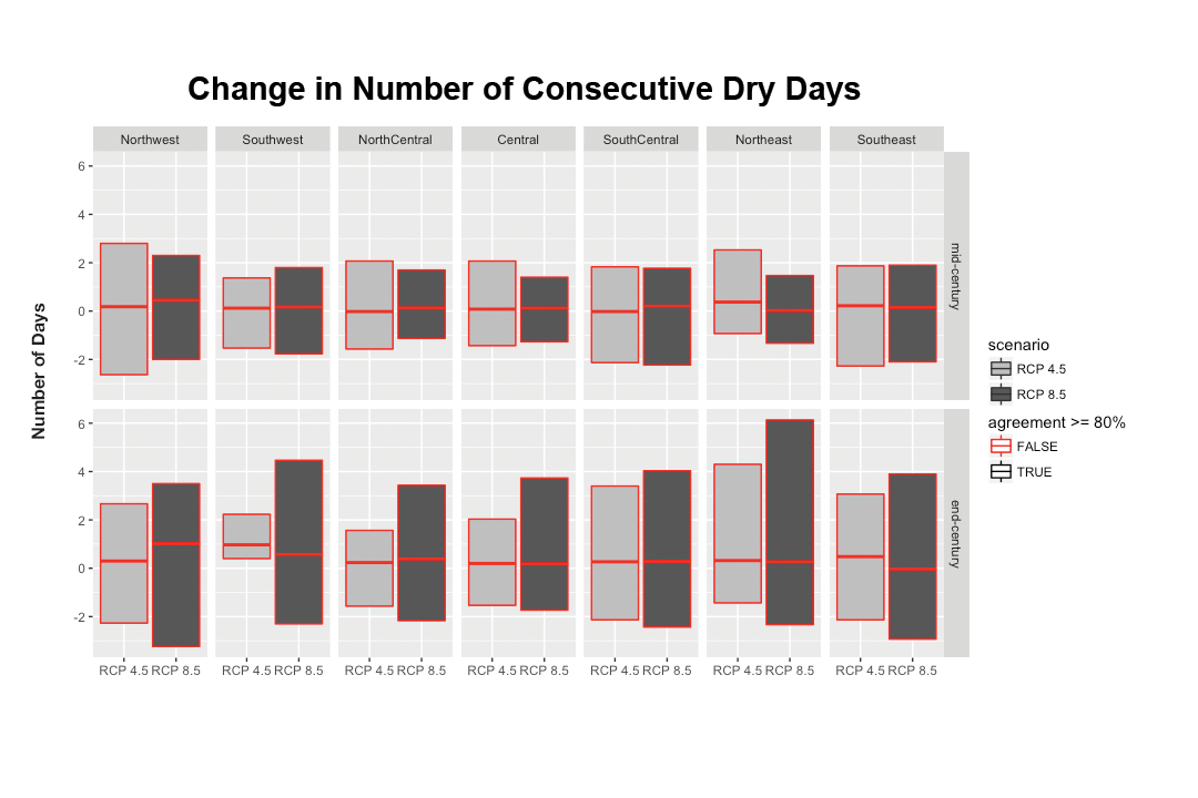
Projected change in wet days
To evaluate changes in wet events, we calculated the number of days/yr where precipitation is greater than 1.0 inch (2.5 cm) and average those values over the period of interest (Figures 2-24).
-
Mid-century projection specifics.—Very modest changes in the number of wet events (i.e., less than 0.5 days) is projected for both emission scenarios. This time, however, model agreement is high that these small changes will occur (approximately 90%).
-
End-of-century projection specifics.—Very high model agreement (approximately 100%) exists that the number of days/yr with precipitation above 1.0 inch (2.5 cm) will increase, although the magnitude of change is still small (less than 1.0 day). The northwestern climate division is projected to have the largest changes in this metric for both emission scenarios, reaching almost a 1.0 day increase of over 1.0 inch (2.5 cm) of precipitation for the period from 2070 to 2099. The range of model output is higher in the business-as-usual emission scenario.
|
|
| Figure 2-24. Graphs showing the increase in the number of wet days/yr projected for each climate division in both stabilization (RCP4.5) and business-as-usual (RCP8.5) emission scenarios. The top row shows projections for mid century (2040-2069) and the bottom row shows projections for end-of-century (2070-2099). The outline of each box is determined by model agreement on the sign of the change (positive or negative). A black outline means there is ≥80% model agreement and a red outline indicates <80% model agreement. Model agreement for the trend of wet days each year was greater than 80%, except for the northeastern climate division. |
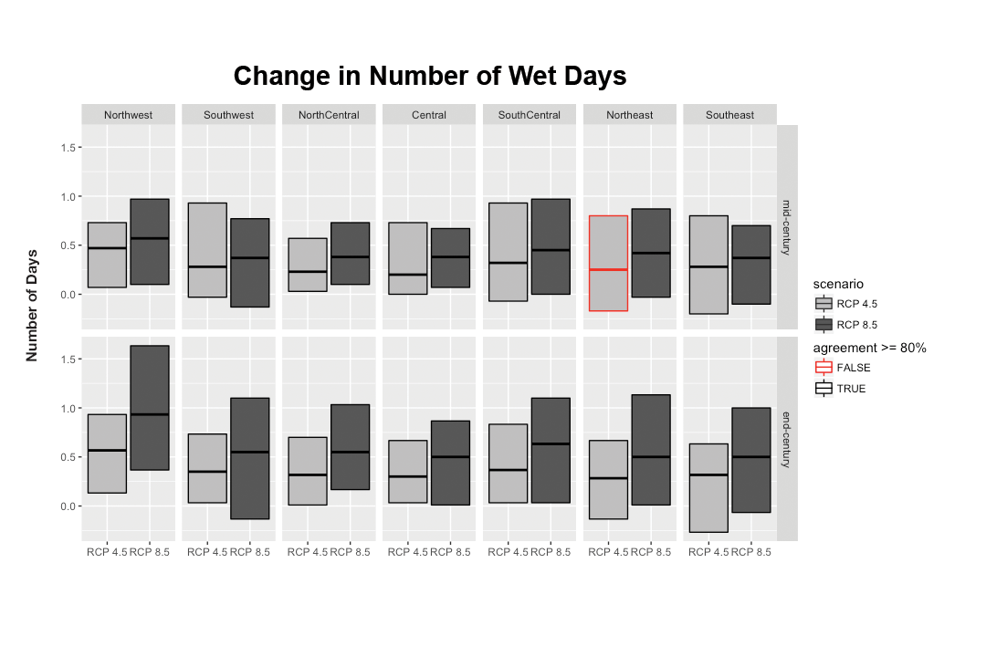
Summary
In mid-century and end-of-century projections, average annual precipitation and variability increase across the state, as does winter, spring, and fall precipitation. Summers, however, show slight decreases in precipitation. The projections suggest little change in the annual frequency of dry and wet events, although there is high uncertainty in the case of wet events. Similar analysis using different metrics for the larger region surrounding Montana indicates an even larger potential (30%) for more days of extreme precipitation (NCA 2014). Overall, the differences in precipitation resulting from the different emission scenarios (i.e., stabilization versus business-as-usual) are small when compared to the impact of the emission scenarios on the temperature projections. Uncertainty in the projections generally increases the further out in time (i.e., in the end-of-century projections), as well as for the higher business-as-usual emission scenario.
KEY KNOWLEDGE GAPS
- Additional climate variables.—Our analysis provides a critical local look at changes for two important climate variables, precipitation and temperature. However, Montana’s climate and its impacts go beyond these. A more in depth downscaling effort that involves physics based models will be required to evaluate two additional important variables, evapotranspiration and drought.
- Land use and land cover change.—Most climate analyses do not account for changes in land cover with climatic trends. However, interactions between climate, vegetation cover, and land use quality are tightly coupled. For example, with changes in temperature and precipitation, ecosystems within Montana may shift to drier conditions resulting in changes to vegetation types. This would contribute to a difference in evapotranspiration rates and aridity.
- Precipitation timing and form.—We took a first look at changes in Montana’s precipitation. However, it is well known that the timing (winter versus spring and summer) and form (rain versus snow) of Montana’s precipitation is critical for areas such as water, forests, and agriculture resources. More work that incorporates physically based, distributed hydrological models is required to understand how our precipitation distribution will change in both space (low elevations to mountaintops) and time.
CONCLUSIONS
The analysis presented in this chapter shows that Montana has warmed—up to 2.7°F (1.5°C) annually as averaged across the state—since 1950. Seasonally, that warming has been greatest in winter (3.9°F [2.2°C]) and spring (2.6°F [1.4°C]). Montana’s number of frost days has decreased by 12 days since 1951. Statewide, average annual precipitation did not change between 1950 and 2015, although variations caused by global climate oscillations, such as El Niño events, explain some of the historical precipitation variability in parts of the state.
With this historical context, we considered Montana’s future under two potential greenhouse gas emission scenarios. Using those scenarios, we employed standard modeling techniques available to climate scientists today—ensembles of general circulation models—and projected Montana’s climate over the next century. Our analyses focused on projecting the possible range of temperature and precipitation amounts in Montana, under our chosen greenhouse gas emission scenarios.
While the model results varied, one message is imminently clear: Montana in the coming century will be a warmer place.
One thing is clear: Montana in the coming century will be a warmer place.
In Table 2-6 we provide a summary of the work done and described in this chapter (plus in accompanying appendices). In summary, Montana is projected to continue to warm in all geographic locations, seasons, and under all emission scenarios throughout the 21st century. By mid century, Montana temperatures are projected to increase by up to 6°F (3°C); by the end of the century, temperatures will increase by up to 9.8°F (5.4°C) (both projections depend on the particular carbon emission scenario [i.e., RCP], and these numbers are based on the business-as-usual [RCP8.5] scenario). Projections show that we could have up to 70 more frost-free days at the end of the century. Likewise, frequency of extreme heat will increase. In eastern Montana, for example, we may have as many as 54 days/yr in which maximum temperatures exceed 90°F (32°C).
In mid- and end-of-century projections, average annual precipitation and variability increase across the state, as do winter, spring, and fall precipitation. Summer months, however, show small decreases in precipitation. Current projections suggest little change in the frequency of dry and wet events, although projections in the former case show high uncertainty.
Montanans must be prepared for projected increases in temperature in the future. Because of its interior location, Montana has warmed more over the last 65 yr than the national average, and it will experience greater warming than most parts of the country in the future, particularly when compared to states in coastal regions. Key to the concern is that coming temperature changes will be larger in magnitude and occur more rapidly than any time since our 1889 declaration of statehood (and, to be sure, well before).
Montana’s average annual temperature is projected to increase through the end-of-century for all models, all emission scenarios, and in all geographic locations.
Changes in temperature and precipitation associated with climate change will undoubtedly impact Montana’s water resources, forestry, and agriculture. These changes will have direct impacts on all Montanans, as we explore in subsequent chapters of this assessment.
| Climate Metric— | Trend and future scenario |
| Atmospheric CO2 concentrations | Global atmospheric carbon dioxide concentrations have increased over 100 ppm since Montana statehood and are projected to increase under both future scenarios considered here. |
| Average temperature | Since 1950, average statewide temperatures have increased by 0.5°F/decade (0.3°C/decade), with greatest warming in spring; projected to increase by 3-7°F (1.7-3.9°C) by mid century, with greatest warming in summer and winter and in the southeast. |
| Maximum temperatures | Maximum temperatures have increased most in spring and are projected to increase 3-8°F (1.7-4.4°C) by mid century, with greatest increases in August and in the southeast. |
| Days above 90°F (32°C) | Extreme heat days are projected to increase by 5-35 additional days by mid century, with greatest increases in the northeast and south. |
| Minimum temperatures | Minimum temperatures have increased most in winter and spring and are projected to increase 3-7°F (1.7-3.9°C) by mid century, with greatest increases in January and in the southeast. |
| Frost-free days | Frost-free days are projected to increase by 24-44 days by mid century, particularly in the west. |
| Average precipitation | Statewide precipitation has decreased in winter ( 0.14 inches/decade [-0.36 cm/decade]) since 1950, but no significant change has occurred in annual mean precipitation, probably because of very slight increases in spring and fall precipitation. Precipitation is projected to increase, primarily in spring (0.2-0.7 inches [0.5-1.8 cm]) in the northwest; a slight statewide decrease in summer precipitation and increased year-to-year variability of precipitation are projected, as well. |
| Number of consecutive dry days | Little projected change, with a maximum increase of 3 days to -3 days under the most severe scenario by end of the century. However, increased variability in precipitation suggests potential for more severe droughts, particularly in connection with climate oscillations. |
| Number of consecutive wet days | No substantial change projected. |
RECOMMENDED FURTHER READING
Abatzoglou JT, Brown TJ. 2012. A comparison of statistical downscaling methods suited for wildfire applications. International Journal of Climatology 32:772–80.
[IPCC] Intergovernmental Panel on Climate Change. 2014. In: Pachauri RK, Meyer LA, editors. Climate Change 2014: synthesis report; contribution of working groups I, II and III to the Fifth Assessment Report of the Intergovernmental Panel on Climate Change. Geneva Switzerland: IPCC. 151 p.
Kunkel KE, Stevens LE, Stevens SE, Sun L, Janssen E, Wuebbles D, Kruk MC, Thomas DP, Shulski MD, Umphlett NA, and 7 more. 2013. Regional climate trends and scenarios for the US National Climate Assessment: Part 4. Climate of the US Great Plains. Washington DC: National Oceanic and Atmospheric Administration. NOAA Technical Report NESDIS 142-4. 91 p.
Pederson GT, Graumlich LJ, Fagre DB, Kipfer T, Muhlfeld CC. 2009. A century of climate and ecosystem change in western Montana: what do temperature trends portend? Climatic Change 98(1):133–54.
Trenberth KE. 2011. Changes in precipitation with climate change. Climate Research 47:123–138.
LITERATURE CITED
Abatzoglou JT. 2013. Development of gridded surface meteorological data for ecological applications and modelling. International Journal of Climatology 33:121–31.
Abatzoglou JT, Brown TJ. 2012. A comparison of statistical downscaling methods suited for wildfire applications. International Journal of Climatology 32:772–80.
Cayan DR, Dettinger MD, Kammerdiener SA, Caprio JM, Peterson DH. 2001. Changes in the onset of spring in the western United States. Bulletin of the American Meteorological Society 82:399–415.
Clarke L, Edmonds J, Jacoby H, Pitcher H, Reilly J, Richels R. 2007. Scenarios of greenhouse gas emissions and atmospheric concentrations. Sub-Report 2.1a of synthesis and assessment product 2.1 by the US Climate Change Science Program and the Subcommittee on Global Change Research. Washington DC: Department of Energy, Office of Biological & Environmental Research. 164 p. Available online http://www.climatescience.gov/Library/sap/sap2-1/finalreport/default.htm. Accessed 2017 May 10.
CLIMDEX. [undated]. CLIMDEX—datasets for indices of climate extremes [website]. Available online http://climdex.org/. Accessed 2017 Mar 6.
[CMIP5] Coupled Model Intercomparison Project. [undated]. Overview [website]. Available online http://cmip-pcmdi.llnl.gov/. Accessed 2017 Mar 18.
Dang H, Gillett NP, Weaver AJ, Zwiers FW. 2007. Climate change detection over different land surface vegetation classes. International Journal of Climatology 27:211–20.
Davy R, Esau I. 2016. Differences in the efficacy of climate forcings explained by variations in atmospheric boundary layer depth. Nature Communications 7:11690. doi:10.1038/ncomms11690.
Dettinger MD, Cayan DR. 1995. Large-scale atmospheric forcing of recent trends toward early snowmelt runoff in California. Journal of Climate 8:606–23.
Dightman RA. 1963. -70°F in Montana. Weatherwise 16:272-3.
Forster P, Ramaswamy V, Artaxo P, Berntsen T, Betts R, Fahey DW, Haywood J, and 45 more. 2007. Changes in atmospheric constituents and in radiative forcing [chapter]. In: Solomon S, Qin D, Manning M, Chen Z, Marquis M, Averyt KB, Tignor M, Miller HL, editors. Climate change 2007: the physical science basis. Cambridge UK: Cambridge University Press. p 129-234.
Fujino J, Nair R, Kainuma M, Masui T, Matsuoka Y. 2006. Multi-gas mitigation analysis on stabilization scenarios using Aim Global Model. Energy Journal 27:343–53.
Global Climate Observing System. [undated]. GCOS essential climate variables [website]. Available online http://www.wmo.int/pages/prog/gcos/index.php?name=EssentialClimateVariables. Accessed 2017 Mar 6.
Guttman NB, Quayle RG. 1996. A historical perspective of US climate divisions. Bulletin of the American Meteorological Society 77:293–303.
[IPCC] Intergovernmental Panel on Climate Change. 2013a. In: Stocker TF, Qin D, Plattner G-K, Tignor M, Allen SK, Boschung J, Nauels A, Xia Y, Bex V, Midgley PM, editors. Climate Change 2013: the physical science basis. Contribution of working group I to the Fifth Assessment Report of the Intergovernmental Panel on Climate Change. Cambridge UK and New York NY, USA: Cambridge University Press. 1535 p.
[IPCC] Intergovernmental Panel on Climate Change. 2013b. Data distribution center—what is a GCM? [webpage] Available online http://www.ipcc-data.org/guidelines/pages/gcm_guide.html. Accessed 2017 Mar 6.
[IPCC] Intergovernmental Panel on Climate Change. 2014. In: Pachauri RK, Meyer LA, editors. Climate Change 2014: synthesis report; contribution of working groups I, II and III to the Fifth Assessment Report of the Intergovernmental Panel on Climate Change. Geneva Switzerland: IPCC. 151 p.
Karl T, Koss WJ. 1984. Regional and national monthly, seasonal, and annual temperature weighted by area, 1895-983. Historical Climatology Series 4-3. Asheville NC: National Climatic Data Center. 38 p.
Leathers DJ, Brent Y, Palecki MA. 1991. The Pacific/North American teleconnection pattern and United States climate. Part I: Regional temperature and precipitation associations. Journal of Climate 4:517–28.
Liebmann B, Dole RM, Jones C, Bladé I, Allured D. 2010. Influence of choice of time period on global surface temperature trend estimates. Bulletin of American Meteorological Society 91:1485-91. doi:org/10.1175/2010BAMS3030.1.
[MACA] Multivariate adaptive constructed analogs. [undated]. MACA statistically downscaled
climate data from CMIP5 [website]. Available online http://maca.northwestknowledge.net/. Accessed 2016 Oct 16.
Mann ME, Bradley RS, Hughes MK. 1999. Northern Hemisphere temperatures during the past millennium: inferences, uncertainties, and limitations. Geophysical Research Letters 26 (6):759–62.
Mantua NJ, Hare SR. 2002. The Pacific Decadal Oscillation. Journal of Oceanography 58(1):35–44.
Mote PW, Hamlet AF, Clark MP, Lettenmaier DP. 2005. Declining mountain snowpack in western North America. Bulletin of the American Meteorological Society 86(1):39–49.
[NAS] National Academy of Sciences. 2011. America’s climate choices. Washington DC: The National Academies Press. 134 p.
[NAS] National Academy of Sciences. [undated]. Climate change at the National Academies [website]. Available online https://nas-sites.org/americasclimatechoices/more-resources-on-climate-c.... Accessed 2017 Mar 6.
[NASA] National Aeronautics and Space Administration. [undated]. NASA data [website]. Available online https://mynasadata.larc.nasa.gov/glossary/earths-energy-budget-2/. Accessed 2017 Mar 6.
[NCA] National Climate Assessment. 2014. In: Melillo JM, Richmond T, Yohe GW, editors. Climate change impacts in the United States: the third national climate assessment. Washington DC: US Global Change Research Program. 841 p. doi:10.7930/J0Z31WJ2.
[NOAAa] National Oceanic and Atmospheric Administration. [undated]. US climate divisions [website]. Available online https://www.ncdc.noaa.gov/monitoring-references/maps/us-climate-division.... Accessed 2017 Mar 6.
[NOAAb] National Oceanic and Atmospheric Administration. [undated]. Climate normals [website]. Available online https://www.ncdc.noaa.gov/data-access/land-based-station-data/land-based.... Accessed 2017 Mar 6.
[NOAAc] National Oceaic and Atmorspheric Administration. [undated]. Climate at a glance [website]. Available online: www.ncdc.noaa.gov/cag/. Accessed 2017 Mar 6.
[NWSa] National Weather Service. [undated]. Climate prediction center—El Niño and La Niña winter features over North America [website]. Available online http://www.cpc.ncep.noaa.gov/products/analysis_monitoring/ensocycle/nawi.... Accessed 2017 Mar 6.
[NWSb] National Weather Service. [undated]. Montana El Niño precipitation and temperature rankings [website]. Available online http://www.cpc.ncep.noaa.gov/products/analysis_monitoring/ensostuff/stat.... Accessed 2017 Mar 6.
Oyler JW, Ballantyne A, Jencso K, Sweet M, Running SW. 2015. Creating a topoclimatic daily air temperature dataset for the conterminous United States using homogenized station data and remotely sensed land skin temperature. International Journal of Climatology 35:2258–79.
Riahi K, Grübler A, Nakicenovic N. 2007. Scenarios of long-term socio-economic and environmental development under climate stabilization. Technological Forecasting and Social Change 74(7):887–935.
Stewart IT, Cayan DR, Dettinger MD. 2005. Changes toward earlier streamflow timing across western North America. Journal of Climate 18:1136–55.
Stocker TF, Qin D, Plattner G-K, Tignor M, Allen SK, Boschung J, Nauels A, Xia Y, Bex V, Midgley PM, editors. 2013. Climate change 2013: the physical science basis. Contribution of working group I to the fifth assessment report of the Intergovern¬mental Panel on Climate Change. Cambridge UK and New York NY: Cambridge University Press. 1535 p.
[USGCRP] US Global Change Research Program. [undated]. Glossary [website]. Available online http://www.globalchange.gov/climate-change/glossary. Accessed 2017 Mar 6.
van Vuuren DP, Edmonds J, Kainuma M, Riahi K, Thomson A, Hibbard K, Hurtt GC, Kram T, Krey V, Lamarque J-F, Masui T, Meinshausen M, Nakicenovic N, Smith SJ, Rose SK. 2011. The representative concentration pathways: an overview. Climatic Change 109:5. doi:10.1007/s10584-011-0148-z.
Vose RS, Applequist S, Durre I, Menne MJ, Williams CN, Fenimore C, Gleason K, Arndt D. 2014. Improved historical temperature and precipitation time series for US climate divisions. Journal of Applied Meteorology and Climatology 53(5):1232-51. Available online http://dx.doi.org/10.1175/JAMC-D-13-0248.1. Accessed 2017 May 10.
Wilhite DA. 2000. Drought as a natural hazard: concepts and definitions [chapter]. In: Wilhite DA, editor. Drought: a global assessment, Vol. I. London: Routledge. p 3–18.